The imos method
The basics: the 1-dimensional, 0-degree imos method
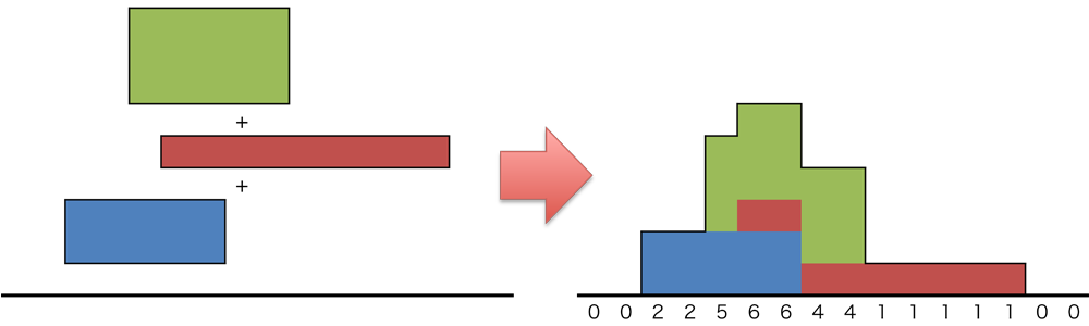
Figure 1: An image of adding a 0-degree function on a one-dimensional line
Example problem
Naive solution
for (int i = 0; i < T; i++) table[i] = 0;
for (int i = 0; i < C; i++) {
  // For each time from S[i] to E[i] - 1, increment the count by 1
  for (int j = S[i]; j < E[i]; j++) {
    table[j]++;
  }
}
// Find the maximum
M = 0;
for (int i = 0; i < T; i++) {
  if (M < table[i]) M = table[i];
}
Solution using the imos method
for (int i = 0; i < T; i++) table[i] = 0;
for (int i = 0; i < C; i++) {
  table[S[i]]++;  // Arrival: increment the count by 1
  table[E[i]]--;  // Departure: decrement the count by 1
}
// Simulate
for (int i = 0; i < T; i++) {
  if (0 < i) table[i] += table[i - 1];
}
// Find the maximum
M = 0;
for (int i = 0; i < T; i++) {
  if (M < table[i]) M = table[i];
}
Extension to more dimensions
The greatest feature of the imos method is that, compared with the naive approach, it scales well as the number of dimensions grows. You cannot escape the curse of dimensionality, so applying it in very high dimensions is difficult; but two- and three-dimensional problem settings are extremely common, and the imos method is useful in those situations.Example problem
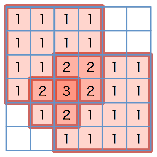
Figure 2: The rectangles (in red) where monsters appear, and
the number of monster kinds appearing on each tile
the number of monster kinds appearing on each tile
Naive solution
for (int y = 0; y < H; y++) {
  for (int x = 0; x < W; x++) {
    tiles[y][x] = 0;
  }
}
for (int i = 0; i < N; i++) {
  // Add 1 to the range [(A[i],C[i]), (B[i],D[i])) where monster i appears
  for (int y = C[i]; y < D[i]; y++) {
    for (int x = A[i]; x < B[i]; x++) {
      tiles[y][x]++;
    }
  }
}
// Find the maximum
int tile_max = 0;
for (int y = 0; y < H; y++) {
  for (int x = 0; x < W; x++) {
    if (tile_max < tiles[y][x]) {
      tile_max = tiles[y][x];
    }
  }
}
Solution using the imos method
for (int y = 0; y < H; y++) {
  for (int x = 0; x < W; x++) {
    tiles[y][x] = 0;
  }
}
// Adding the weights (Figure 3)
for (int i = 0; i < N; i++) {
  tiles[C[i]][A[i]]++;
  tiles[C[i]][B[i]]--;
  tiles[D[i]][A[i]]--;
  tiles[D[i]][B[i]]++;
}
// Prefix sum in the horizontal direction (Figures 4, 5)
for (int y = 0; y < H; y++) {
  for (int x = 1; x < W; x++) {
    tiles[y][x] += tiles[y][x - 1];
  }
}
// Prefix sum in the vertical direction (Figures 6, 7)
for (int y = 1; y < H; y++) {
  for (int x = 0; x < W; x++) {
    tiles[y][x] += tiles[y - 1][x];
  }
}
// Find the maximum
int tile_max = 0;
for (int y = 0; y < H; y++) {
  for (int x = 0; x < W; x++) {
    if (tile_max < tiles[y][x]) {
      tile_max = tiles[y][x];
    }
  }
}
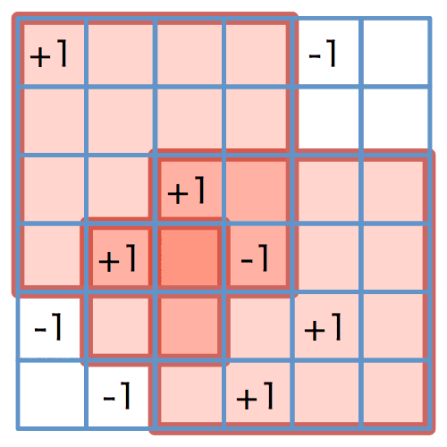
Figure 3: The result of adding the weights
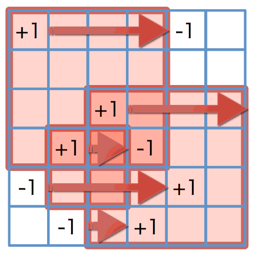
Figure 4: Accumulating in the horizontal direction
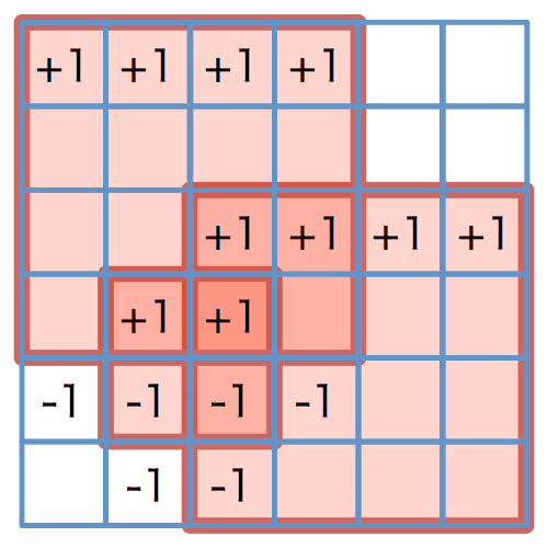
Figure 5: The result of accumulating horizontally
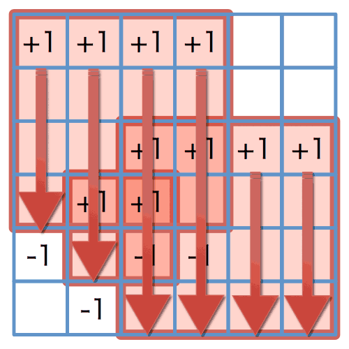
Figure 6: Accumulating in the vertical direction
Figure 7: The result of accumulating vertically
Extension to special coordinate systems
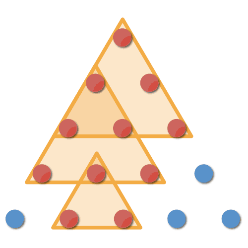
Figure 8: A triangular coordinate system
The differencing technique
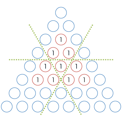
Figure 9: The weights to be filled in
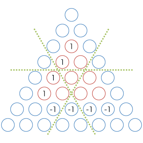
Figure 10: The top-left-to-bottom-right difference of Figure 9
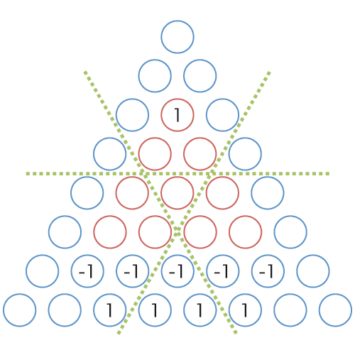
Figure 11: The top-right-to-bottom-left difference of Figure 10
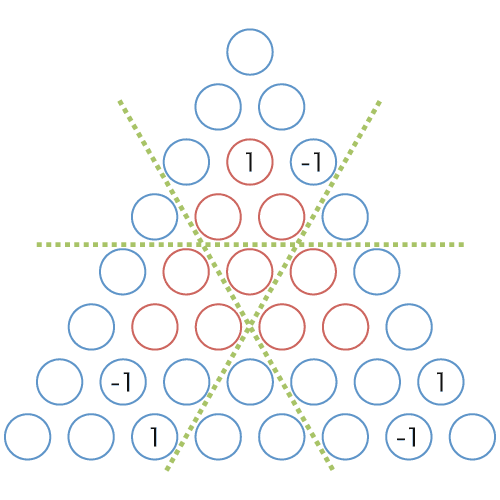
Figure 12: The left-to-right difference of Figure 11
Extension to higher degrees
Differences of a quadratic function
| 0 | 1 | 2 | 3 | 4 | 5 | 6 | 7 | 8 | 9 |
| 0 | 0 | 0 | 1 | 4 | 9 | 16 | 25 | 36 | 49 |
↓difference ↑prefix sum
| 0 | 1 | 2 | 3 | 4 | 5 | 6 | 7 | 8 | 9 |
| 0 | 0 | 0 | 1 | 3 | 5 | 7 | 9 | 11 | 13 |
↓difference ↑prefix sum
| 0 | 1 | 2 | 3 | 4 | 5 | 6 | 7 | 8 | 9 |
| 0 | 0 | 0 | 1 | 2 | 2 | 2 | 2 | 2 | 2 |
↓difference ↑prefix sum
| 0 | 1 | 2 | 3 | 4 | 5 | 6 | 7 | 8 | 9 |
| 0 | 0 | 0 | 1 | 1 | 0 | 0 | 0 | 0 | 0 |
Figure 13: Differences of the quadratic function (x-2)_+^2
Gaussian functions and the imos method

Equation 1: The Gaussian function (left) and its approximation (right)
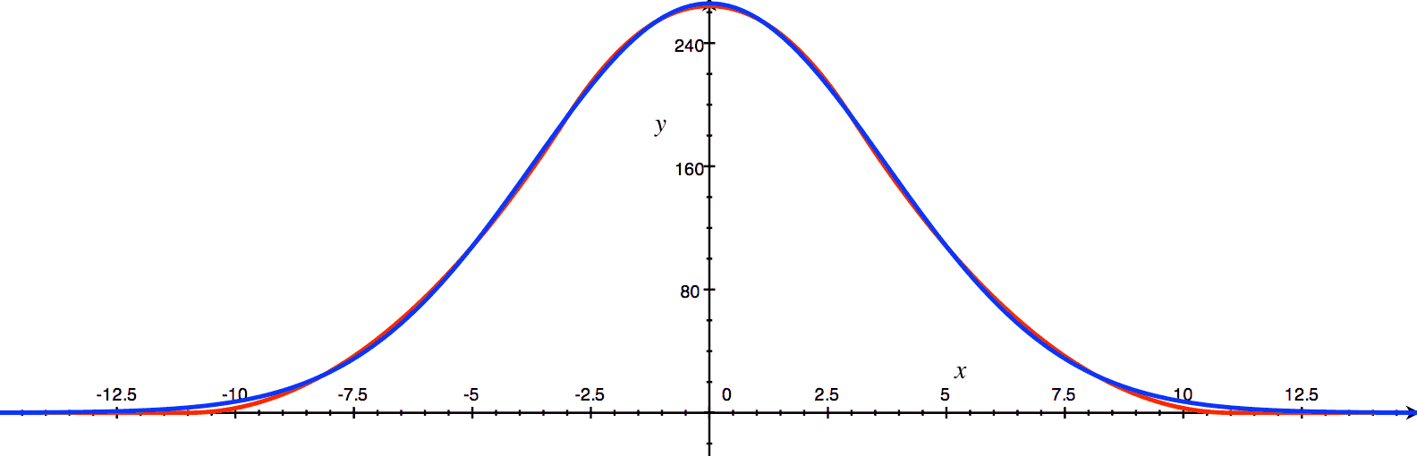
Figure 14: The Gaussian function (blue) and its polynomial approximation (red)
| -12 | -11 | -10 | -9 | -8 | -7 | -6 | -5 | -4 | -3 | -2 | -1 | 0 | 1 | 2 |
| 0 | 0 | 3 | 3 | 0 | 0 | 0 | 0 | 0 | 0 | -11 | -11 | 0 | 0 | 0 |
↓prefix sum ↑difference
| -12 | -11 | -10 | -9 | -8 | -7 | -6 | -5 | -4 | -3 | -2 | -1 | 0 | 1 | 2 |
| 0 | 0 | 3 | 6 | 6 | 6 | 6 | 6 | 6 | 6 | -5 | -16 | -16 | -16 | -16 |
↓prefix sum ↑difference
| -12 | -11 | -10 | -9 | -8 | -7 | -6 | -5 | -4 | -3 | -2 | -1 | 0 | 1 | 2 |
| 0 | 0 | 3 | 9 | 15 | 21 | 27 | 33 | 39 | 45 | 40 | 24 | 8 | -8 | -24 |
↓prefix sum ↑difference
| -12 | -11 | -10 | -9 | -8 | -7 | -6 | -5 | -4 | -3 | -2 | -1 | 0 | 1 | 2 |
| 0 | 0 | 3 | 12 | 27 | 48 | 75 | 108 | 147 | 192 | 232 | 256 | 264 | 256 | 232 |
Figure 15: The Gaussian function approximated by the imos method
| -12 | -11 | -10 | -9 | -8 | -7 | -6 | -5 | -4 | -3 | -2 | -1 | 0 | 1 | 2 |
| 1 .49 | 3 .42 | 7 .28 |
14 .41 | 26 .57 | 45 .58 | 72 .76 | 108 .08 |
149 .41 | 192 .20 | 230 .09 | 256 .31 | 265 .70 |
256 .31 | 230 .09 |
Figure 16: The target Gaussian function to be approximated
Appendix
Problems where the imos method can be used
- [Easy] Osaki … 1-dimensional 0-degree imos method, ACM-ICPC Japan Alumni Group Practice Contest for Japan Domestic 2007 - [AOJ]
- [Easy] Nails … 0-degree imos method on triangular coordinates, Japanese Olympiad in Informatics 2012 Final Round Problem 4 - [AOJ]
- [Medium] Paint Colors … coordinate compression + 2-dimensional 0-degree imos method + breadth-first search (depth-first search is also possible depending on stack capacity), Japanese Olympiad in Informatics 2008 Final Round Problem 5 - [AOJ]
- [Medium] Plugs … 2-dimensional 0-degree imos method + ad hoc, Japanese Olympiad in Informatics 2010 Training Camp Day 4 Problem 4
- [Hard] Pyramid … first-degree imos method on a special coordinate system, Autumn Fest 2012: I