A Numerically Stable and Fast Implementation of Moving Averages and Variances

This article presents a method for computing the mean and variance of the most recent \(w\) points at each time step in a series while satisfying three conditions simultaneously: (1) the computational cost is \(O(T)\), independent of the window width \(w\); (2) the computation uses only cumulative sums and elementwise operations, making it fully vectorizable; and (3) it remains numerically stable regardless of the level or drift of the series. We first show how to compute moving sums and averages stably using per-chunk cumulative sums (§1). We then extend the same chunk structure to moving variances (§2). The building blocks are classical: Welford's online algorithm[1] and its generalization, the merge formula of Chan et al.[2] Here we show how to combine them for moving-window computation. A PyTorch implementation is available through the msum and mvar functions in qfeval-functions, a library we are developing.

The basic idea has three parts.

Moving sum: If we split the series into chunks of length \(w\), every window decomposes into at most two parts: a suffix of the previous chunk and a prefix of the current chunk. Cumulative sums let us compute the sums of all prefixes and suffixes of every chunk at once. Combining them gives the moving sum and moving average (§1).
Moving variance (per-part statistics): For each part, instead of retaining only its sum, we retain a triple: its count, mean, and sum of squared deviations. We compute these statistics from deviations relative to an element of the part itself (the first or last value of the chunk). Because variance is invariant under translation, this keeps the error at the scale of local variation within the window without changing the result (§2.3).
Moving variance (merging statistics): We combine the variance statistics of the two parts using the merge formula of Chan et al. to obtain the statistics for the complete window (§2.4).

At the heart of the method is the following merge formula. Given two disjoint subsets \(A\) and \(B\), with respective counts \(n_A\) and \(n_B\), means \(\mu_A\) and \(\mu_B\), and sums of squared deviations \(M_A\) and \(M_B\), where \(M = \sum (x - \mu)^2\), we have

\[ \boxed{\;M_{A\cup B} = M_A + M_B + \frac{n_A\,n_B}{n_A + n_B}\,\delta^2,\qquad \delta = \mu_B - \mu_A\;} \]

as derived in §2.4. The moving variance is \(\mathrm{Var} = M_{A\cup B}/(w - \mathrm{ddof})\). By expressing both the decomposition and the merge as tensor operations, we can compute the moving variance at every time step using only four cumulative sums and elementwise operations.

\(\mathrm{ddof}\) (delta degrees of freedom) specifies the amount subtracted from the count in the variance denominator. The notation follows the argument name used by numpy and pandas. Use \(\mathrm{ddof} = 1\) for the sample (unbiased) variance and \(0\) for the population variance (§2.4).

Problem setting

Given a series \(x_1, \dots, x_T\) of length \(T\) and a window width \(w\), we compute the sum, mean, and variance of the most recent window \((x_{t-w+1}, \dots, x_t)\) at each time step \(t\). The output has the same length as the input. The first \(w-1\) entries, whose windows would reach back before the start of the series, are NaN; any entry whose window contains a NaN is also NaN. This matches the convention used by pandas' rolling(w).

Financial time series present a combination of conditions under which naive implementations can easily run into accuracy or performance problems. For example, price levels (e.g., \(10^4\) to \(10^6\)) may be orders of magnitude larger than their fluctuations (around \(1\)), while float32, with roughly 7 significant digits, is commonly used on GPUs. Moreover, a single batch may contain thousands of series, each with hundreds of thousands of time steps. We therefore require the following four properties.

\(O(T)\) computational cost: The running time should not depend on the window width \(w\). For daily data, long windows such as \(w = 250\) are commonly used.
Vectorizable: The whole computation should consist of tensor operations (cumulative sums and elementwise operations), with no explicit sequential loop along the time axis. This allows efficient execution on GPUs and with SIMD.
Numerically stable: The error should be governed by the scale of local variation within the window, not by the level, drift, or length of the series.
Exact propagation of NaN and ±inf: A missing value or infinity should affect only the windows that contain it, and should not affect the results of windows that do not.

The first two requirements can be met by a naive formula, while the third can be met by recomputing each window from scratch. Satisfying all four simultaneously, however, requires some care. We first examine why the naive moving sum loses accuracy on long series and stabilize it through chunking (§1). We then extend this structure to moving variance (§2).

1. Moving sums and averages: chunked cumulative sums

Before tackling moving variance, let us consider the moving sum. Because the moving average is simply the moving sum divided by \(w\), we focus on the sum below.

1.1. Differencing a global cumulative sum loses accuracy as the series grows

A common way to compute a moving sum in \(O(T)\) is to take the difference between two values of a global cumulative sum, \(S_t - S_{t-w}\), where \(S_t = \sum_{i \le t} x_i\). However, this method loses accuracy as the series grows. For a series with level \(\mu\), \(S_t \approx t\mu\) becomes large, and merely representing it as a floating-point number incurs an absolute error of about \(\varepsilon\, t\,|\mu|\). Here \(\varepsilon\) is the unit roundoff, about \(6 \times 10^{-8}\) for float32. Because the true window sum is on the order of \(w\mu\), the relative error is of order \(\varepsilon\, t/w\) and grows toward the end of the series. With float32, \(t = 10^7\), and \(w = 100\), this error reaches 0.6%.

This error cannot be avoided simply by improving the algorithm used to compute the cumulative sum. Whether we use sequential or pairwise addition, once the computed \(S_t\) is rounded to a single floating-point number, it carries a representation error of about \(\varepsilon\,|S_t|\) in the best case. If \(S_t\) and \(S_{t-w}\) have the same sign and are close in value, the subtraction itself can be exact (by Sterbenz's lemma). However, both operands already differ from their true values by about \(\varepsilon\,t\,|\mu|\), and these errors remain significant relative to the much smaller true value \(w\mu + O(w\sigma)\). The chunking introduced in the next section can also be viewed as limiting each cumulative sum to at most \(w\) terms, thereby curbing this error growth.

1.2. Chunking: every window splits into at most two parts

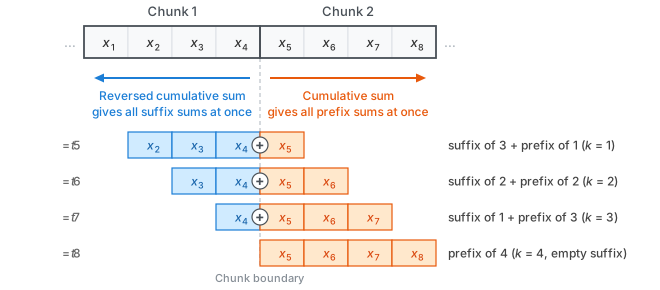
Prepend at least \(w\) NaNs to the series, adding enough to make the total length a multiple of \(w\) (see §6 for why at least \(w\) are needed), and then split the padded series into chunks of length \(w\). Because the window and the chunks have the same length, every window spans at most two consecutive chunks. Specifically, a window ending inside chunk \(c\) is the concatenation of a suffix of chunk \(c-1\) and a prefix of chunk \(c\):

\[ \text{window} = \underbrace{\text{suffix of chunk } c-1}_{A\ (\text{length } w - k)}\ +\ \underbrace{\text{prefix of chunk } c}_{B\ (\text{length } k)} \qquad (1 \le k \le w) \]

When \(k = w\), the prefix is the entire chunk and the suffix is empty. For each chunk, the sums of all prefixes of lengths 1 through \(w\) can be computed at once with a cumulative sum from the beginning. Likewise, the sums of all suffixes can be computed at once with a reversed cumulative sum. There are \(T/w\) chunks, and each cumulative sum costs \(O(w)\) per chunk, so the total cost is \(O(T)\).

Window decomposition by chunking (w = 4). The four windows ending inside chunk 2 each split into a suffix of chunk 1 (blue) and a prefix of chunk 2 (orange); a single addition across the chunk boundary gives the window sum. Suffix sums are computed at once with a reversed cumulative sum, prefix sums with a cumulative sum. — Figure 1: Window decomposition by chunking (\(w = 4\)) Every window decomposes into a suffix of the previous chunk and a prefix of the current chunk. A single addition of the suffix and prefix sums gives the window sum. The sums of all parts are computed at once using cumulative sums in both directions within each chunk (blue and orange arrows).

1.3. From part sums to moving sums and moving averages

The window sum is obtained by adding the suffix sum and the prefix sum. Because each part sum contains at most \(w\) terms, the error remains within \(O(\varepsilon w)\) times the scale of the local values. Unlike the error from the global cumulative sum (§1.1), it does not depend on the series length \(T\). Moreover, the computation uses only tensor operations—forward and reversed cumulative sums, plus elementwise additions—with no explicit sequential loop. The msum and ma functions in qfeval-functions use this approach.

Simply adding the part sums, however, is not enough to obtain the variance. Variance is a nonlinear quantity based on the sum of squared deviations from the mean, and the reference mean differs from one window to the next. In the next section, we replace the sum retained for each part with a set of variance statistics.

2. Extending the method to moving variance

A well-known way to obtain variance uses two moving sums, but it is numerically unstable (§2.1). Existing numerically stable alternatives either require more computation or cannot be vectorized along the time axis (§2.2). In this section, we reuse the chunk structure from §1, replacing each part's sum with variance statistics. The resulting moving variance has the same properties as the moving sum: \(O(T)\) cost, vectorizability, and error governed by local variation.

2.1. The sum-of-squares formula suffers cancellation when the data level is large

A commonly used \(O(T)\) method is the "sum-of-squares formula," which derives the variance from two moving sums of \(x\) and \(x^2\):

\[ \mathrm{Var} = \frac{1}{w - \mathrm{ddof}}\left(\sum_{i} x_i^2 - \frac{\bigl(\sum_{i} x_i\bigr)^2}{w}\right) \]

Consider a window with mean \(\mu\) and variance \(\sigma^2\). This formula extracts the small value \(w\sigma^2\) by subtracting two large numbers, \(\sum x^2 \approx w(\mu^2 + \sigma^2)\) and \((\sum x)^2/w \approx w\mu^2\). Because the relative rounding error of each term is of order \(\varepsilon\), the relative error of the result can reach roughly \(\varepsilon\,(1 + \mu^2/\sigma^2)\). For float32 data with \(\mu = 10^6\) and \(\sigma = 1\), the error is amplified by a factor of \(6 \times 10^4\), leaving no significant digits. Rounding often makes the difference negative, so taking its square root to obtain the moving standard deviation yields NaN. Measurements confirm that accuracy degrades as this estimate predicts (§3.3). Even computing the moving sums stably using the method in §1 cannot eliminate the cancellation in this subtraction. The problem lies not in how the moving sums are computed, but in the sum-of-squares formula itself.

Both \(\sum x^2\) and \((\sum x)^2/w\) have magnitude about \(w(\mu^2 + \sigma^2)\). Merely representing each as a floating-point number incurs an absolute error of about \(\varepsilon\, w \mu^2\). Meanwhile, the true value of the difference is \(w\sigma^2\), so the relative error grows to order \(\varepsilon\,\mu^2/\sigma^2\). The \(1 +\) term captures the fact that even when \(\mu = 0\), rounding alone leaves a relative error of \(\varepsilon\).

2.2. Stable alternatives sacrifice speed or vectorizability

Recomputing each window independently yields numerically stable results. For example, one can use the two-pass method (first compute the mean, then the sum of squared deviations) or Welford's method. However, both cost \(O(Tw)\). In PyTorch, they can be implemented by creating a view of every window with unfold and applying var. In our environment, this approach was 8 to 300 times slower than the \(O(T)\) methods (§4). Because its running time is proportional to the window width, it becomes impractical when \(w\) reaches several hundred.

Another approach is a sequential update that adds the element entering the window and removes the one leaving it (an add/remove variant of Welford's method). It costs \(O(T)\) and is reasonably stable numerically. pandas' rolling uses this method. However, because the state at each time step depends on the previous state, the computation cannot be parallelized along the time axis. Here we assume batches of thousands of series processed in float32, so we instead use tensor operations that can also be parallelized along that axis.

2.3. Per-part statistics and local centering

Let us return to the chunking from §1.2. To compute the variance, we retain three values for each part: its count \(n\), mean \(\mu\), and sum of squared deviations \(M = \sum (x - \mu)^2\). Deriving a prefix's \(M\) from cumulative sums requires the sum-of-squares formula, and applying that formula directly would reintroduce the cancellation described in §2.1. We therefore apply it to deviations obtained by subtracting a reference value from each value in the chunk. Let the reference value be \(r\) and define \(y_i = x_i - r\). Because variance and \(M\) are invariant under translation, the following equations hold for any reference value \(r\):

\[ S = \sum_i y_i,\qquad Q = \sum_i y_i^2,\qquad \bar m = \frac{S}{n},\qquad M = Q - \frac{S^2}{n},\qquad \mu = r + \bar m \]

Here \(M = Q - S^2/n\) has the same form as the expression in §2.1, but \(y\) represents a local deviation from the reference value. This prevents cancellation from growing without bound as the level \(\mu\) increases (§3.1). We compute cumulative sums of \(y\) and \(y^2\) for prefixes and reversed cumulative sums for suffixes. These four cumulative sums provide \((n, \bar m, M)\) for every part.

As the reference, we use the first value of the chunk for prefixes and the last value for suffixes. This choice has two advantages.

The error stays at the scale of the window: Every prefix contains the first element, and every suffix contains the last, so the reference value is always an element of the part itself (Figure 2). Because each part is a subset of the window, the magnitude of the deviations \(y\) cannot exceed the range of values within the window. Even when the series has a high level or drift, the computation involves only differences local to the window (Figure 3, §3.1).
The effect of NaN and ±inf is confined exactly: When the reference value is NaN or infinite, it affects only parts that contain that value—that is, precisely the windows whose results should be NaN anyway (§3.2). If an aggregate such as the chunk mean were used instead, a single NaN in the chunk would affect windows that do not contain it.

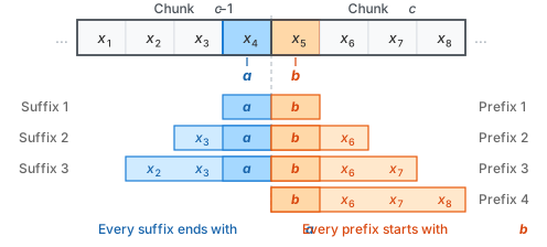
Choice of reference values (w = 4). For two adjacent chunks, all suffixes of lengths 1–3 and all prefixes of lengths 1–4 are laid out. Every suffix contains the chunk's last value a, and every prefix contains the chunk's first value b. a and b are adjacent in the series. — Figure 2: Choice of reference values (\(w = 4\)) Every suffix contains the chunk's last value \(a\), and every prefix contains the chunk's first value \(b\), so the reference is always an element of the part itself. The two reference values \(a\) and \(b\) are adjacent in the series, so \(b - a\) is the difference between adjacent elements (§2.4).

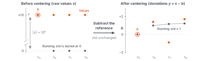
Comparison of scales before and after local centering. On the left, at the raw-value scale, the values lie flat near 10 to the 6th power, and the running standard deviation is indistinguishable from 0. On the right, after subtracting the reference value b, the deviations are around ±2 and the running standard deviation is around 1, both visible at the scale of the window. — Figure 3: Scales before and after local centering (example with level \(10^6\)) The elements \(x_5, \dots, x_8\) of chunk \(c\) (orange) and the running standard deviation at each point (gray), shown as raw values (left) and as deviations after subtracting the reference value \(b = x_5\) (right). At the scale of the raw values, the target standard deviation (≈ 1) is indistinguishable from 0 and cannot be recovered from the difference of the sums of squares in float32, which has about 7 significant digits. After subtracting the reference value, both the deviations and the running standard deviation are represented at the local scale of the window. Translation does not change the standard deviation itself.

2.4. Merging the two parts with the formula of Chan et al.

We combine the statistics of the two parts, \(A\) (the suffix) and \(B\) (the prefix), using the merge formula of Chan et al.[2] introduced above:

\[ M_{A\cup B} = M_A + M_B + \frac{n_A\,n_B}{n_A + n_B}\,\delta^2,\qquad \delta = \mu_B - \mu_A \]

This formula is an identity, not an approximation. When \(n_B = 1\), it reduces to Welford's online update[1]. Let the overall mean be \(\mu = (n_A \mu_A + n_B \mu_B)/(n_A + n_B)\). Each part's contribution then decomposes into variation within the part and variation due to the difference between the part means. The three terms in the formula therefore represent, respectively, the variation within \(A\), the variation within \(B\), and the variation between \(A\) and \(B\).

Let \(n = n_A + n_B\). Squaring \(x - \mu = (x - \mu_A) + (\mu_A - \mu)\) and summing over \(A\), the cross term vanishes because \(\sum_{x \in A}(x - \mu_A) = 0\), giving \(\sum_{x \in A}(x - \mu)^2 = M_A + n_A(\mu_A - \mu)^2\). The same holds for \(B\). Substituting \(\mu_A - \mu = -n_B\delta/n\) and \(\mu_B - \mu = n_A\delta/n\), the additional term becomes \(\delta^2(n_A n_B^2 + n_B n_A^2)/n^2 = \delta^2 n_A n_B/n\), yielding the merge formula.

\(\delta\), too, can be computed from local values alone. Since both part means can be written as "reference value + relative mean," we have

\[ \delta = (b - a) + \bigl(\bar m_B - \bar m_A\bigr) \]

The first term, \(b - a\), is the difference between the two reference values: \(a\) is the last value of chunk \(c-1\), and \(b\) is the first value of chunk \(c\). Thus, they are adjacent elements in the series. Subtracting adjacent elements removes the level of the data, and every subsequent computation involves only local differences. For windows with \(k = w\), the suffix is empty, so we simply use the \(M_B\) of the prefix that spans the entire chunk. Finally, the variance is

\[ \mathrm{Var}_t = \frac{M_{A \cup B}}{w - \mathrm{ddof}} \]

with \(\mathrm{ddof} = 1\) for the sample variance and \(0\) for the population variance. The moving standard deviation is the square root of this variance.

2.5. The full algorithm

Prepend enough NaNs to make the padded length a multiple of \(w\), and split the result into chunks of length \(w\) (§1.2).
Within each chunk, compute cumulative sums of \(y\) and \(y^2\), where \(y\) is the deviation from the first value. This yields \((n, \bar m, M)\) for every prefix.
Similarly, compute reversed cumulative sums of deviations from the last value to obtain \((n, \bar m, M)\) for every suffix.
For each window, use the merge formula to compute \(M_{A \cup B}\), then divide by \(w - \mathrm{ddof}\). Windows and parts can be matched by simply shifting indices, so this stage also uses only elementwise operations.
The prepended NaNs automatically make the first \(w-1\) outputs NaN. If \(T < w\), every output is NaN.

The four cumulative sums are the only operations with dependencies along the time axis. A cumulative sum is a primitive that can be implemented as a parallel scan, even on GPUs. In PyTorch, the method takes about 30 lines and uses only forward and reversed cumulative sums plus elementwise operations (see mvar in qfeval-functions).

Although a cumulative sum may appear inherently sequential, arranging partial sums in a tree allows each chunk to be processed in parallel with depth \(O(\log w)\). This operation is called a prefix scan and is widely used to implement cumsum on parallel hardware.

2.6. A small numerical example

Let \(x = (50, 48, 49, 51, 52)\) and \(w = 3\). Prepend 4 NaNs (written as ∅ below) to obtain a length of 9, then split the result into three chunks:

\[ [\,∅,\ ∅,\ ∅\,]\quad[\,∅,\ 50,\ 48\,]\quad[\,49,\ 51,\ 52\,] \]

The window \((48, 49, 51)\) ending at \(x_4 = 51\) splits into the suffix \(A = (48)\) of chunk 2 and the prefix \(B = (49, 51)\) of chunk 3.

Part	Reference value	Deviations \(y\)	\(n\)	\(\bar m\)	\(M\)	\(\mu\)
\(A = (48)\)	last value 48	\((0)\)	1	0	0	48
\(B = (49, 51)\)	first value 49	\((0, 2)\)	2	1	\(4 - 2^2/2 = 2\)	50

The reference values are adjacent elements, so their difference is \(49 - 48 = 1\). Thus, \(\delta = 1 + (1 - 0) = 2\), and the merge formula gives

\[ M_{A \cup B} = 0 + 2 + \frac{1 \cdot 2}{3} \cdot 2^2 = \frac{14}{3},\qquad \mathrm{Var} = \frac{14/3}{3 - 1} = \frac{7}{3} \]

Computing the sum of squared deviations directly from the mean \(148/3\) also gives \(16/9 + 1/9 + 25/9 = 14/3\), as expected. Even if we add \(10^6\) to the entire series, every value used in this computation—including the difference of \(1\) between the reference values—remains unchanged, apart from quantization when the inputs are rounded to floating-point numbers. This is the effect of local centering.

3. Numerical stability properties

3.1. Why the error stays at the local scale of the window

Cancellation can occur when each part computes \(M = Q - S^2/n\). However, because the reference value is an element of the part itself, the magnitude of each deviation \(y\) cannot exceed the range \(R\) of the values within the window. The population variance of \(w\) points with range \(R\) has the lower bound \(\sigma^2 \ge R^2/(2w)\), because the two endpoints of the range alone contribute at least \(R^2/2\) to the sum of squared deviations. The number of digits lost in the subtraction is therefore bounded. The relative error is at worst \(O(\varepsilon w^2)\) and is usually much smaller. It is also independent of the level \(\mu\), drift, and length \(T\) of the series. In contrast, the error factor \(\mu^2/\sigma^2\) in the sum-of-squares formula (§2.1) grows without bound as the level increases.

Since \(|y| \le R\), we have \(Q = \sum y^2 \le wR^2\). The absolute error in the cumulative sums of \(S\) and \(Q\), together with the subsequent operations, is at worst \(O(\varepsilon w^2 R^2)\). Meanwhile, the true value is \(M = w\sigma^2 \ge R^2/2\), so the relative error is bounded by \(O(\varepsilon w^2)\). In measurements (§3.3) using float32 with \(w = 20\)–\(50\), the error attributable to the algorithm remained below \(10^{-6}\). The per-window two-pass and Welford methods have error \(O(\varepsilon w)\); for extremely large windows where the last digit matters, the two-pass method has an advantage (§7).

Moreover, when all values in the window are equal, the deviations \(y\) are exactly 0, so the variance is exactly 0 with no rounding error. The sum-of-squares formula incurs rounding error even for constant windows and can produce negative values.

3.2. Why the influence of NaN and ±inf is confined to the window

The property that “the result is NaN if and only if the window contains a NaN or infinity” holds exactly. For a window containing neither, the result is bit-for-bit identical to the result obtained after replacing NaNs and infinities elsewhere in the series with finite values. This property follows from choosing an element of each part as its reference value. The implementation's tests place NaN and ±inf at each time step in turn and verify the property at every position (§6).

A NaN or infinity can propagate through three paths. (1) Each part's cumulative sums: a cumulative sum up to a given position does not depend on later elements. The statistics of prefixes ending before the offending value and suffixes starting after it are therefore unaffected. (2) The reference values: the first value of a chunk, used as the reference for prefixes, belongs to every prefix. Likewise, the chunk's last value, used as the reference for suffixes, belongs to every suffix. Thus, if a reference value is NaN or infinite, the part necessarily contains that value. (3) The two reference values used to compute \(\delta\) in the merge formula also belong to the suffix and prefix, respectively. Consequently, the affected range consists exactly of the windows that contain the NaN or infinity.

3.3. Measurements

Using float32, we compared the accuracy of this method with that of the sum-of-squares formula (§2.1). The reference results were computed from the same series in float64. “Offset” is a random series with mean \(10^6\) and variance 1 (\(w = 20\)). “Drift” is a random walk around a level of 1000, with small steps having a standard deviation of 0.01 (\(w = 50\)). The latter illustrates a case in which subtracting a single global constant does not improve accuracy.

Case (float32)	Sum-of-squares formula	This method
Offset: relative error (median)	about \(9 \times 10^{4}\) (no significant digits remain)	\(6 \times 10^{-3}\) (input quantization error is the floor)
Offset: fraction of negative variances	31%	0
Drift: relative error (median)	about \(72\)	\(1.3 \times 10^{-4}\)

The remaining error in this method comes mainly from quantizing the inputs to float32. Near \(10^6\), adjacent float32 values are about 0.06 apart. When compared with reference results computed in float64 from the same float32 inputs, the error attributable to the algorithm itself was below \(10^{-6}\) in both cases.

4. Speed

The sum-of-squares formula uses two cumulative sums and elementwise operations, whereas this method uses four cumulative sums and additional elementwise operations. Per-window recomputation (unfold + var), meanwhile, costs \(O(Tw)\), and its running time grows in proportion to the window width. The following results were measured in our environment using an Apple silicon CPU, PyTorch 2.7, and float32.

Shape	Window	Sum-of-squares formula	Per-window recomputation	This method
(10000,)	20	0.21 ms	1.5 ms	0.18 ms
(100, 10000)	20	2.0 ms	145 ms	2.7 ms
(100, 10000)	500	2.1 ms	763 ms	3.1 ms
(1000, 10000)	500	21 ms	7237 ms	23 ms

This method takes 0.9 to 1.5 times as long as the sum-of-squares formula, and its running time changes little as the window width grows from 20 to 500. Within the range shown in the table, it is 8 times faster than per-window recomputation for a single series and 50 to 300 times faster for batches. The method is also well suited to GPUs, although the table reports only CPU results; we have not benchmarked GPU performance.

5. Comparison with related methods

Welford's online algorithm[1] stably updates the mean and variance statistics as elements are added one at a time. The formula of Chan et al.[2] generalizes it by allowing any two subsets to be merged. This formula has traditionally been used for parallel computation and pairwise aggregation. Our method combines it with a chunking scheme in which every moving window splits into at most two parts, allowing all time steps to be processed in a single batch of tensor operations. It can also be viewed as a single-level adaptation of pairwise summation—which reduces rounding error in sums through block decomposition—to moving windows. The approaches differ as follows.

Pairwise summation splits a sequence in half and recursively computes the sum of each half. With sequential addition, rounding errors can accumulate in proportion to the number of terms \(T\); with pairwise summation, they remain roughly proportional to the depth \(\log T\) of the addition tree. This standard technique is used by numpy's sum, among others.

Method	Cost	Vectorizable	Numerical stability
Sum-of-squares formula (two moving sums)	\(O(T)\)	Yes	Unstable (error factor \(\mu^2/\sigma^2\))
Difference of a global cumulative sum	\(O(T)\)	Yes	Degrades in proportion to series length (§1.1)
Per-window recomputation	\(O(Tw)\)	Yes	Stable (\(O(\varepsilon w)\))
Sequential add/remove (pandas, etc.)	\(O(T)\)	Not along the time axis	Mostly stable (depends on the removal implementation)
This method (chunking + local centering + merge)	\(O(T)\)	Yes	Stable (worst case \(O(\varepsilon w^2)\); independent of level and series length)

Chan et al.[3] and Higham's textbook[4] survey numerically stable methods for computing variance, including the conditions under which each formula loses accuracy and the use of a shift close to the data. The local centering in our method automatically selects such a shift for each part. This choice also confines the effect of a NaN exactly to the windows that contain it (§2.3).

6. Implementation notes

The role of the prepended NaNs: Using NaNs as the padding needed to align chunk boundaries satisfies the output conventions—“the first \(w-1\) outputs are NaN” and “all outputs are NaN if \(T < w\)”—without special-case branches. Prepending at least \(w\) NaNs ensures that even the start of the real data has a preceding chunk.
Handling ddof: We assume \(0 \le \mathrm{ddof} < w\). Typically it is \(1\) for the sample variance or \(0\) for the population variance.
Moving average and moving standard deviation: The moving sum and moving average require only the chunk sums of §1. The moving standard deviation is obtained as the square root of the moving variance.
Clamping negative values: In this method, \(M\) can become slightly negative because of rounding error, whereas the ordinary two-pass method guarantees nonnegativity. If strict nonnegativity is required—for example, before taking a square root—clamp the final result to a minimum of 0. No negative values were observed under the measurement conditions in §3.3.

Our regression tests continuously verify five aspects of the implementation: (1) for every combination of series length and window width, the results match per-window recomputation regardless of where chunk boundaries fall; (2) for float32 series with a large offset, the relative error against a float64 computation on the same inputs remains below a threshold (§3.3); (3) the same holds for random-walk series; (4) when NaN and ±inf are placed at each time step in turn, their effects remain confined to windows containing the offending value (§3.2); and (5) constant windows return exactly 0 while preserving the dtype.

7. Design limitations

The error bound is larger than that of the two-pass method: The worst-case error is \(O(\varepsilon w^2)\), a bound \(w\) times larger than the \(O(\varepsilon w)\) bound of the per-window two-pass method. When last-digit accuracy matters more than speed, or when \(M\) must be guaranteed nonnegative, the two-pass method is preferable (§3.1, §6).
Not suited to streaming: This method assumes batch computation in chunks. For low-latency processing of data that arrives one point at a time, Welford's method or the add/remove approach (§2.2) is more appropriate.
Cannot ignore NaNs within a window: If a window contains a NaN, its result is NaN. Computing over only the non-NaN elements, as with pandas' min_periods, would require a different construction that also tracks the number of valid elements.
Inputs must be floating-point numbers: Because the method prepends NaNs and computes deviations, integer series must first be converted to floating point.

8. Summary

Moving sums obtained by differencing a global cumulative sum lose accuracy as the series grows. By splitting the series into chunks as long as the window, we ensure that every window consists of at most two parts: a suffix and a prefix. Because each part sum contains at most \(w\) terms, moving sums and averages can be computed stably.
Computing moving variance with the sum-of-squares formula amplifies error in proportion to \(\mu^2/\sigma^2\). Stable per-window recomputation, meanwhile, costs \(O(Tw)\), and sequential updates cannot be parallelized along the time axis. Our method replaces the single sum retained for each part with its count, mean, and sum of squared deviations. By expressing these statistics as deviations from an element of the part itself, the entire computation uses only local differences; the two parts are then combined using the merge formula of Chan et al.
The method simultaneously achieves \(O(T)\) cost independent of window width, an implementation using only tensor operations, error independent of the level, drift, and length of the series, and exact propagation of NaNs and infinities. In our measurements, it took 0.9 to 1.5 times as long as the sum-of-squares formula.
The building blocks are the classical methods of Welford and Chan–Golub–LeVeque, published from the 1960s through the 1980s. Here we have shown how to combine them for tensor computation over moving windows. The implementation is available through the msum and mvar functions in qfeval-functions.

9. References

The following are the original sources for the online update and merge formulas, along with standard references on the numerical error analysis of variance computation.

[1] B. P. Welford, "Note on a Method for Calculating Corrected Sums of Squares and Products," Technometrics 4(3), 419―420, 1962. (Welford's online update formula. Stable updates of the mean and sum of squared deviations under sequential insertion)
[2] Tony F. Chan, Gene H. Golub, Randall J. LeVeque, "Updating Formulae and a Pairwise Algorithm for Computing Sample Variances," COMPSTAT 1982, 30―41, 1982. (The update formulas and pairwise algorithm by Chan–Golub–LeVeque. The original source of the merge formula in this article)
[3] Tony F. Chan, Gene H. Golub, Randall J. LeVeque, "Algorithms for Computing the Sample Variance: Analysis and Recommendations," The American Statistician 37(3), 242―247, 1983. (Error analysis and recommendations for variance computation algorithms by the same authors, including the effect of shifting (centering))
[4] Nicholas J. Higham, "Accuracy and Stability of Numerical Algorithms, Second Edition," Society for Industrial and Applied Mathematics, 2002. (The standard textbook on rounding error analysis. Error bounds for summation and variance computation)

Last Modified: July 16, 2026