A long-term investment strategy using the Nikkei average
The Nikkei average was 2,402 yen on January 5, 1970, and 17,451 yen on December 30, 2014 (source: Nikkei Stock Average Data Room). This means that if you had kept investing in line with the Nikkei average, you would have made a 626% profit, which works out to an annual return of 5.8%.
Investing in stocks is on average positive, but this high rate of return is also thanks to the (largely unrepeatable) rapid economic growth and the bubble economy. On the other hand, events such as the collapse of the bubble and the Lehman shock can also turn the return negative.
Investment carries risk, but considering that consumer prices in 2014 had risen to 3.10 times their 1970 level (source: Consumer Price Index, All Items (base index)), simply holding yen also carries risk.
So we consider a way of investing in the Nikkei average that avoids losing assets during recessions as much as possible while still making a profit when possible. Using the daily data from the Nikkei Stock Average Data Room, we look for an investment method that can be expected to make a profit going forward.
The basic strategy
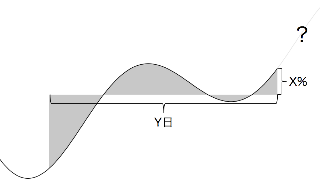
Figure 1: The trend-following strategy
(the state where the price is X% above the average price over the past Y days)
(the state where the price is X% above the average price over the past Y days)
Results of applying the trend-following strategy to the Nikkei average
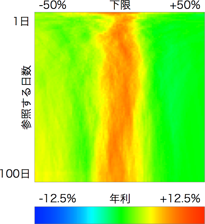
Figure 2: Average return from 1970 to 2014
(The lower bound is multiplied by the square root of the number of years referenced. For example, when the number of referenced days is 1, it shows the range ±50%/√365.0. This is an adjustment based on the fact that the magnitude of fluctuations in prices and the like is proportional to √time.)
(The lower bound is multiplied by the square root of the number of years referenced. For example, when the number of referenced days is 1, it shows the range ±50%/√365.0. This is an adjustment based on the fact that the magnitude of fluctuations in prices and the like is proportional to √time.)
Stability across decades

Figure 3-a: 1970–1979
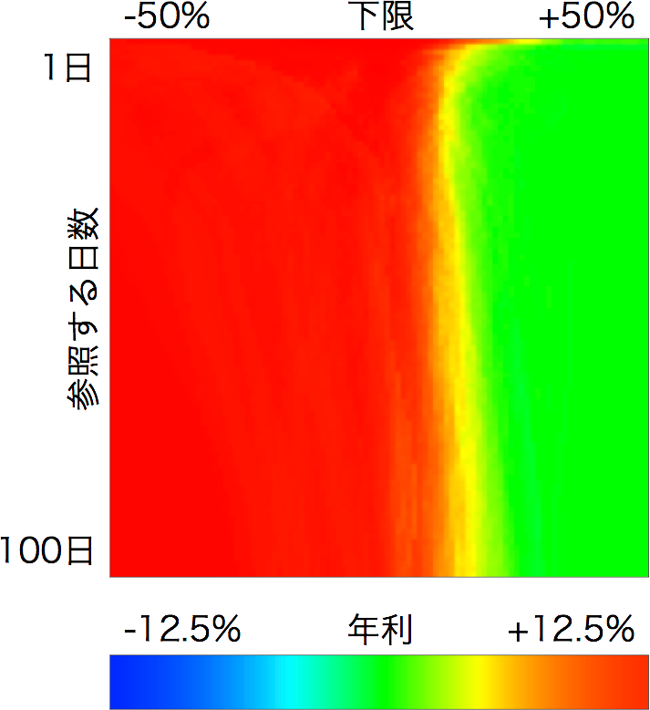
Figure 3-b: 1980–1989
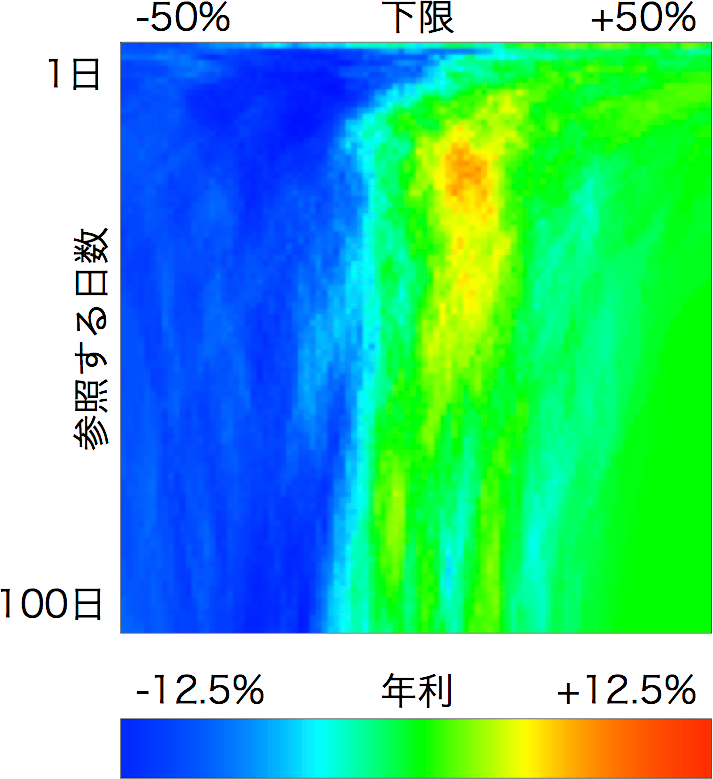
Figure 3-c: 1990–1999
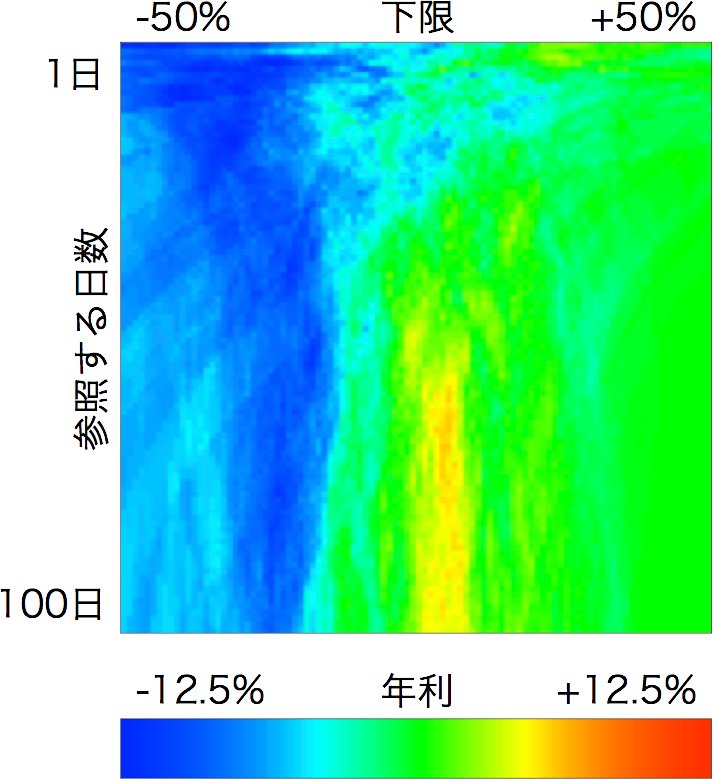
Figure 3-d: 2000–2009
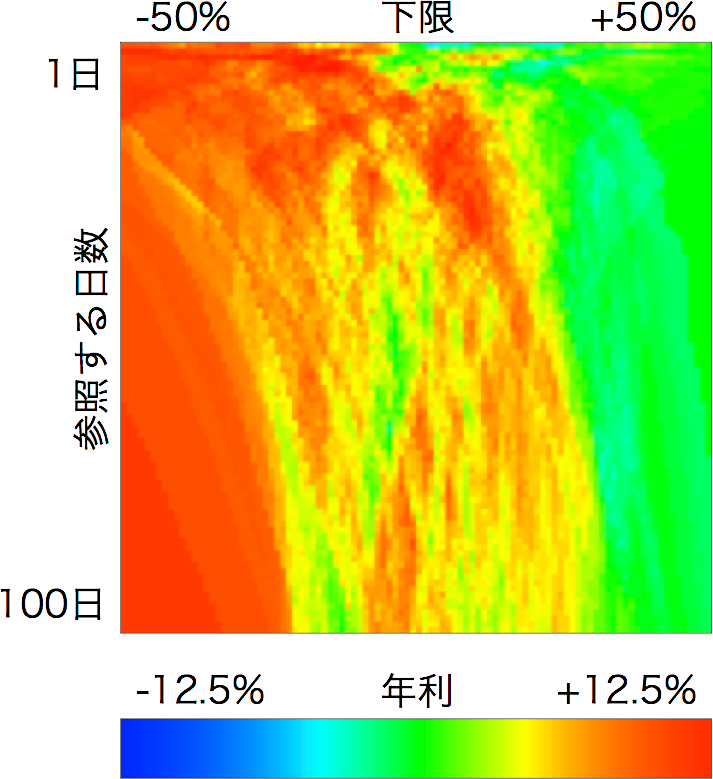
Figure 3-e: 2010–2014
The parameters with the highest rate of return, and the average annual return, were:
Even in the 1990s and 2000s, which were periods of recession, we can see a tendency for the annual return to be positive around where the lower bound is 0.
From Figure 3 we can see, in every decade, a tendency for the annual return not to become small around where the lower bound is 0. This shows that the trend-following strategy may be able to mitigate the risk of recessions.
- 1970s … days: 1, lower bound: -0.05%, annual return 24.7% (Nikkei average's annual return 10.6%),
- 1980s … days: 1, lower bound: +0.15%, annual return 25.5% (Nikkei average's annual return 19.4%),
- 1990s … days: 22, lower bound: +2.38%, annual return 7.6% (Nikkei average's annual return -6.9%),
- 2000s … days: 66, lower bound: +2.06%, annual return 5.8% (Nikkei average's annual return -5.6%),
- 2010s … days: 5, lower bound: -1.77%, annual return 16.1% (Nikkei average's annual return 5.0%).
Day-to-day stability
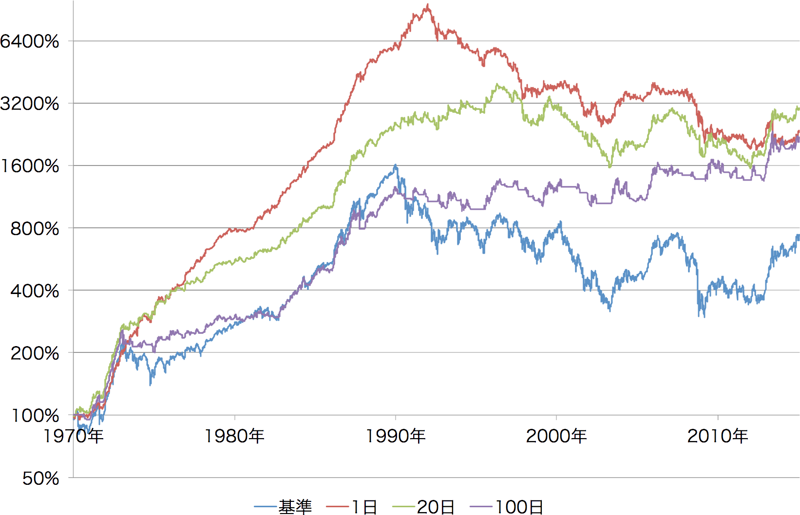
Figure 4: Day-to-day change in assets, with January 1, 1970 set to 1
It shows the change in assets for the Nikkei average and for reference-day counts of 1, 20, and 100 days.
It shows the change in assets for the Nikkei average and for reference-day counts of 1, 20, and 100 days.
Future work
Appendix
- Nikkei Stock Average Data Room … the source of the Nikkei average data
- imos/nikkei (Github) … the crawling program and evaluation program used on this page