Formulating exchange rate fluctuations

To predict exchange rate movements, simply applying machine learning does not provide enough information. So we aim to increase the amount of information and reduce noise by formulating exchange rate fluctuations to some extent.

Examining fluctuations by time of day

Differences between years

If fluctuations by time of day are reliable, we can take them into account in advance. So we investigate how reliable the fluctuations by time of day actually are.

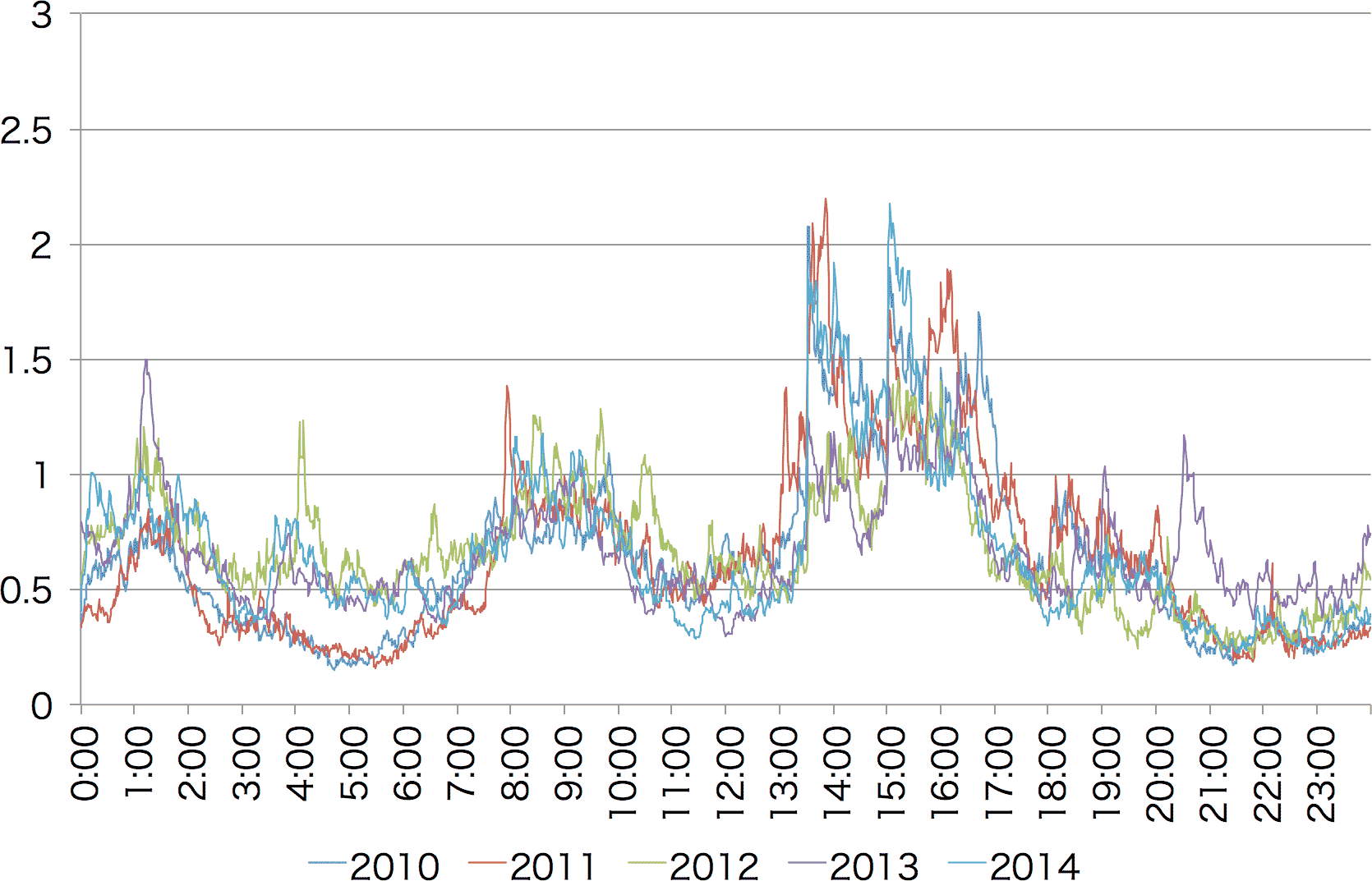
Figure 1: Fluctuation of USD/JPY by time of day during winter time, 2010–2014
(the X axis is the time in UTC, the Y axis is the amount of fluctuation)

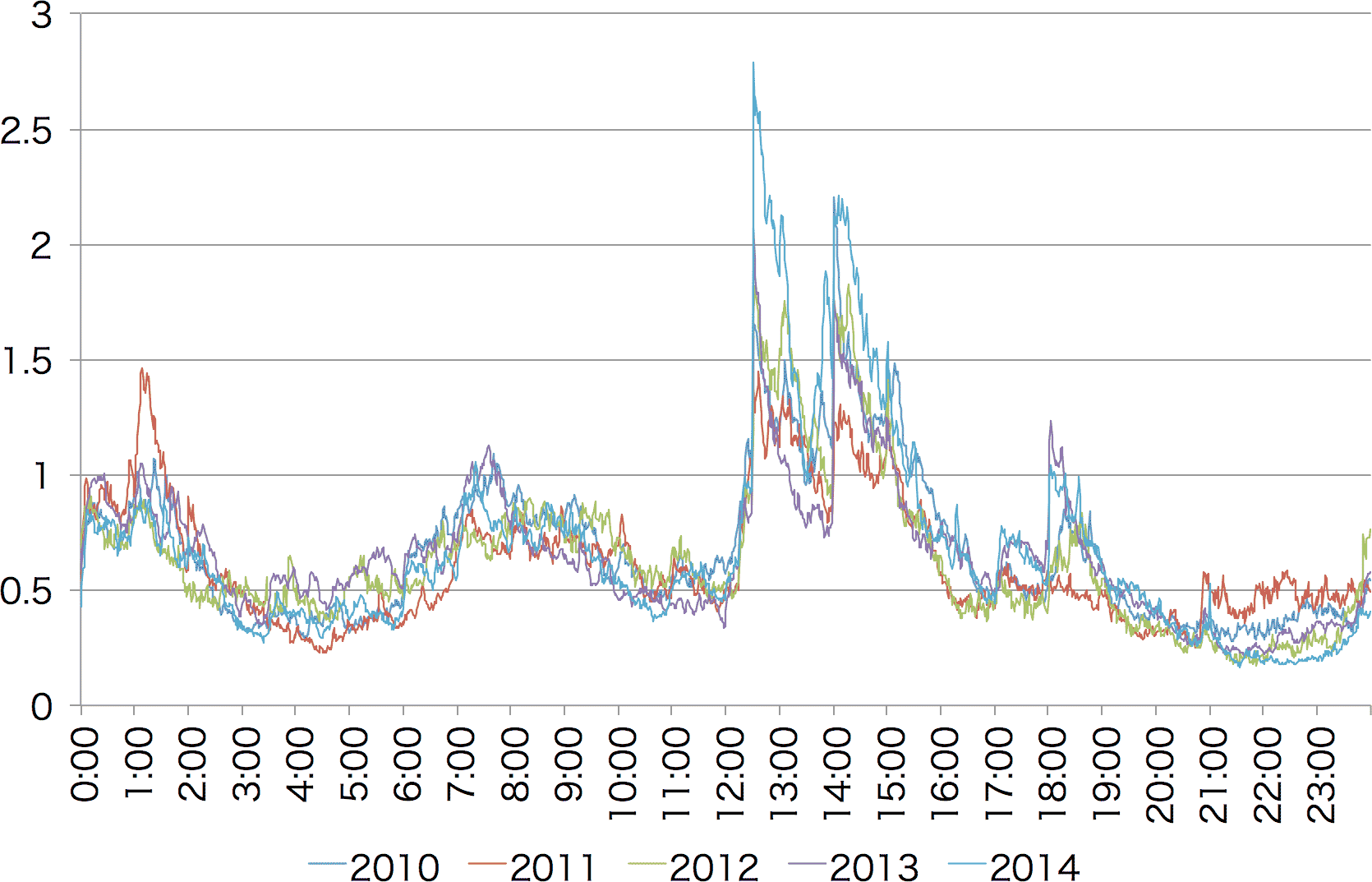
Figure 2: Fluctuation of USD/JPY by time of day during summer time, 2010–2014
(the X axis is the time in UTC, the Y axis is the amount of fluctuation)

Figures 1 and 2 show statistics of the fluctuation of USD/JPY by time of day from 2010 to 2014. Here the amount of fluctuation is defined as the price movement over the past 30 minutes, and we take the median to avoid sudden fluctuations. Because the movement is almost the same from 2010 to 2014, we can see that fluctuations by time of day occur continuously.

Differences by day of the week

When a large fluctuation occurs, being able to distinguish whether it is caused by active trading or by movements in the real economy is important for predicting exchange rates. So we investigate whether there are fluctuations by day of the week and time of day.

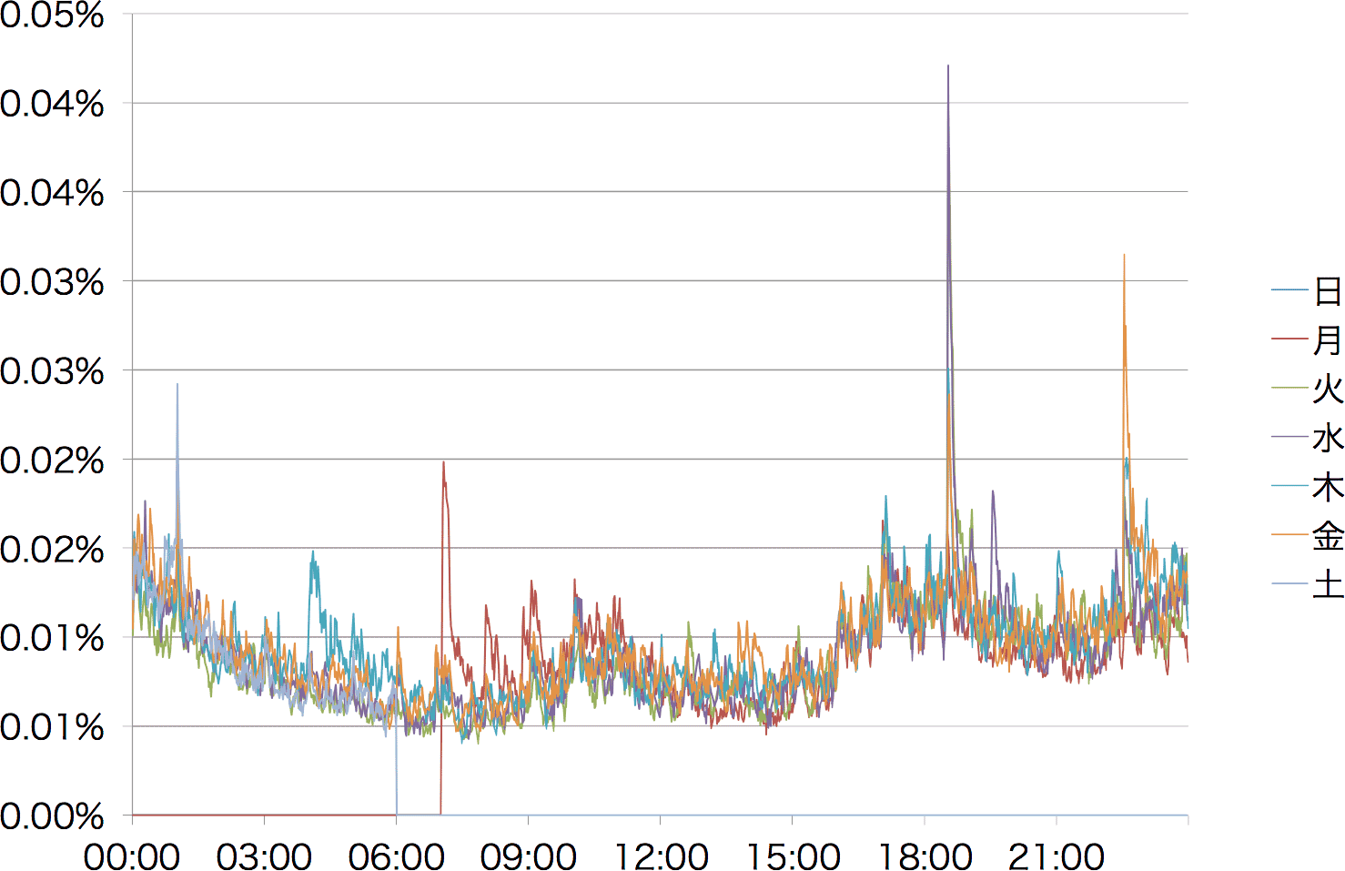
Figure 3: Weekly fluctuation of GBP in 2014
(the X axis is the time, the Y axis is the amount of fluctuation)

Figure 3 shows statistics of the weekly fluctuation of GBP in 2014. Here the amount of fluctuation is defined as the price movement over the past 10 minutes. The sudden fluctuations are considered to be the effects of:

7:00 to 10:00 on Monday … fluctuations that absorb the potential real-economy changes over the weekend
18:30 … fluctuations from the release of UK economic indicators
22:30 … fluctuations from the release of US economic indicators

We can also see that, apart from the start of trading on Monday, there is almost no fluctuation depending on the day of the week.

Examining time and fluctuation scale

Because the electronization of foreign exchange trading has advanced, the history of exchange rate fluctuations that can be used to predict future exchange rates is limited to the past 10 years or so, which cannot be said to be enough for machine learning. If exchange rate fluctuations have a fractal property, it may be possible to increase the data available for learning, so here we examine time and fluctuation scale.

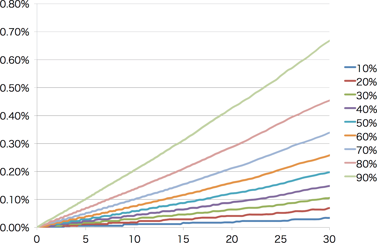
Figure 4: Fluctuation of GBP in 2014
(the X axis is the square root of the target time in minutes, the Y axis is the amount of fluctuation, and each series is the amount of fluctuation that falls within that percentile)

Figure 4 shows statistics of the exchange rate fluctuation of GBP in 2014 (for example, from this graph we can read that a 9-hour fluctuation is 0.50% with 90% probability). Because each series in this graph is almost a straight line, we can see that when time increases by a factor of X, the fluctuation increases by a factor of √X. This matches the relationship between time and fluctuation in a random walk, so it seems reasonable to think that it holds roughly for actual exchange rate fluctuations as well.

Examining fluctuations over time series

When a large fluctuation occurs, if that fluctuation continues to affect subsequent fluctuations, it can be considered that the trading volume itself has changed, which is thought to be noise for technical analysis. So we investigate fluctuations over the time series.

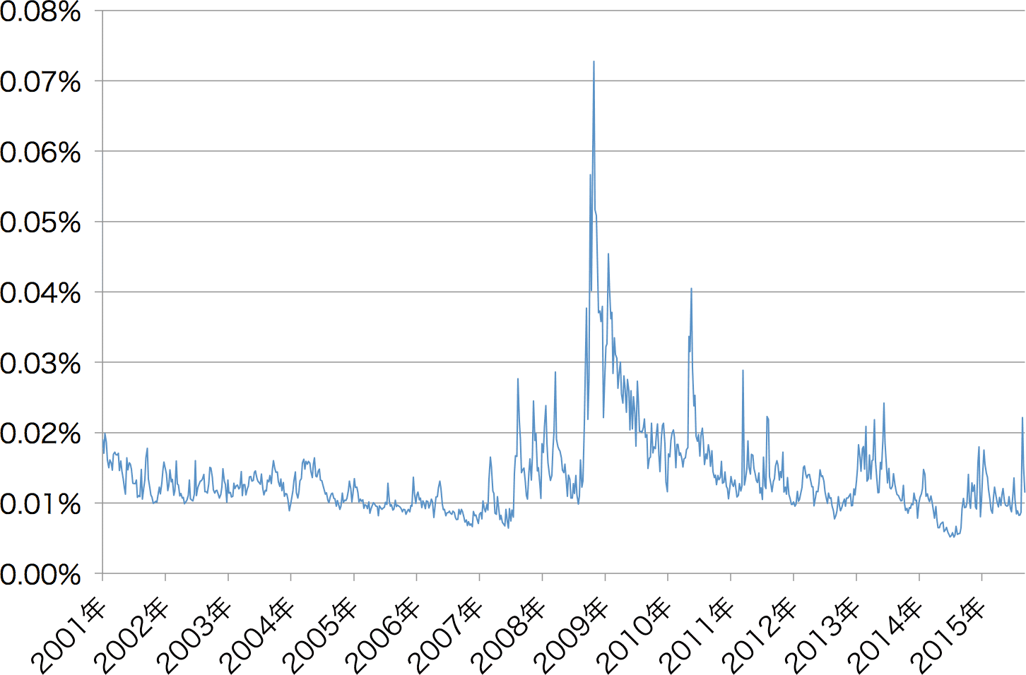
Figure 5: Fluctuation of GBP, 2001–2015

Figure 5 shows the average of the 10-minute fluctuation of GBP taken for each week from 2001 to 2015. Since there were periods of large fluctuation such as from the end of 2008 into 2009, we can see a tendency that once fluctuations become large, they continue to be large.

[Hypothesis] Setting the half-life to about one week gives a good approximation.

Autocorrelation of exchange rate fluctuations

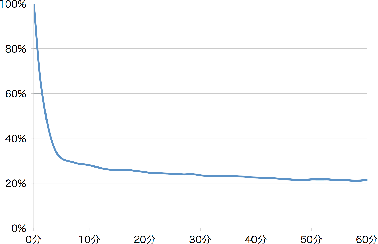
Figure 6: Short-term autocorrelation of GBP in 2014
(the X axis is the time difference, the Y axis is the amount of fluctuation)

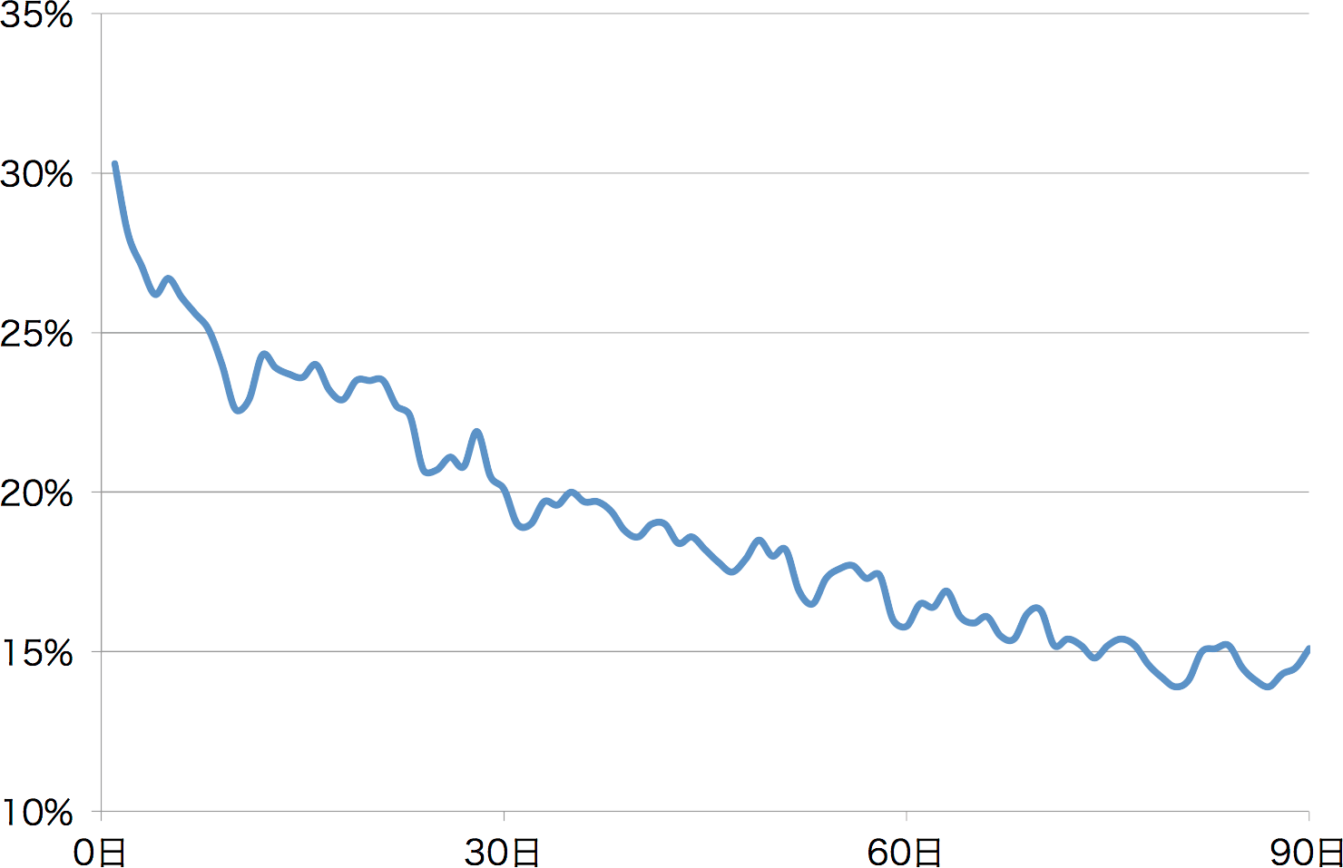
Figure 7: Long-term autocorrelation of GBP, 2001–2014
(the X axis is the time difference, the Y axis is the amount of fluctuation)

Figure 6 shows the average autocorrelation of the 5-minute fluctuation of GBP in 2014 taken within one hour. Figure 7 shows the average autocorrelation of the 30-minute fluctuation of GBP taken within 90 days. Because the correlation in Figure 6 drops sharply as time passes, we can see that short-term fluctuations have almost no effect on trading volume. On the other hand, because the correlation in Figure 7 drops gently, we can consider that trading volume fluctuates gently over a period of several months.