Imos Financial Theory

Published on February 21, 2020

Imos Financial Theory

Because I had never had contact with anyone versed in orthodox financial theory, I came to feel that the direction of my own financial theory differs from it. In this article I therefore explain and organize the fundamental part of that theory so that both people unfamiliar with financial theory and people who understand orthodox financial theory can follow it.
So that you can grasp the overview easily while avoiding leaps in logic, clicking the parts marked with a "blue dashed line" reveals a more detailed explanation.
The parts shown with a blue dashed line give explanations in more general terms for people unfamiliar with financial theory, or provide more detailed explanations of assumptions and equation transformations.

0. Introduction: How Imos Financial Theory Differs from Orthodox Financial Theory

Imos Financial Theory makes it possible to simultaneously derive both "the optimal portfolio composition ratio that is the same answer for every investor" and "the reference amount to invest". If one follows the Capital Asset Pricing Model (CAPM), the composition ratio of the optimal portfolio should be the same for every investor. However, orthodox financial theory often constrains the investable amount to equal one's assets, and the discussion sometimes proceeds as if optimal portfolios with various composition ratios exist along the efficient frontier. In the modern world it is not difficult to buy leveraged products, so this constraint is superfluous. Moreover, modern portfolio theory often assumes that the investor decides the absolute amount of risk they wish to take or the profit they need, but in reality it should be natural to want to take on higher risk if higher returns can be obtained. Imos Financial Theory solves these problems by introducing a logarithmic function as the evaluation function (utility function) for investments that carry a distribution, and conducting all of the discussion on top of it.
Imos Financial Theory is not a theory entirely absent from financial theory, but unlike the orthodox school it aims to optimize an individual's investment strategy, and it assumes that one's own assets are finite and fluctuate greatly depending on the strategy, so the way the discussion is conducted differs. Broadly, it differs in the following two points.
  • As the evaluation function U(x) for investments carrying a distribution (in the language of financial theory, the utility function), we use precisely {\rm ln}(x), and we believe its expected value should be maximized. When performing portfolio optimization, the orthodox school often fixes the expected return (or the volatility) and, within that, minimizes the volatility (or maximizes the expected return) (e.g., Modern portfolio theory - Wikipedia). But from the idea that investors should not fix those quantities but rather take on risk that is worth it, we believe that what should be optimized is the size of the expected return relative to risk. Financial theory too sometimes optimizes the size of the expected return relative to risk by using risk-averse utility functions or the Sharpe ratio, but among these we believe that the logarithmic utility function in particular should be used because of its good properties.
  • As for how to hold financial instruments, we believe that the ratio of each financial instrument to one's own assets (the leverage) should be held fixed. Orthodox financial theory often either limits the quantity of a financial instrument by one's assets, or assumes unlimited borrowing subject to some other constraint, and assumes that over a short period the quantity of the instrument is not changed. But we consider that in reality this has problems—such as being able to trade up to the maximum leverage in margin/credit transactions, and being unable to adequately represent long periods that include rebalancing—so, as a trading model that can be expressed in continuous time including rebalancing, we take the position that "the ratio of each financial instrument to one's own assets (the leverage) should be held fixed."
In this article we use the utility function as an evaluation function of one's own assets. For example, which is preferable—"a bet where with 50% probability your assets halve and with 50% probability your assets double" or "a bet where your assets are certainly multiplied by 1.1"—differs from person to person. This can be rephrased as being determined by that person's utility function. In this example, under the expected value (when a linear function is used as the utility function, i.e. when U(x)=x) the former is rated higher than the latter, U(0.5)×50%+U(2)×50% \gt U(1.1), whereas when the logarithmic function U(x)={\rm ln}(x) is used as the utility function we get U(0.5)×50%+U(2)×50% \lt U(1.1) and the latter is rated higher.
By placing these assumptions, we believe we can resolve a variety of issues—from the problem that under a model constraining one's own assets there is a tendency to preferentially buy real-world leveraged products (and conversely to undervalue stocks with high retained-earnings ratios and low volatility), to the problem that currency overlay products are not highly valued.
In this article we explain these using equations. In Chapter 1, we explain that when a financial instrument with known expected rate of return and volatility exists, the optimal leverage can be determined under the log expected utility. In Chapter 2, we explain that for foreign exchange between stable currencies such as USD/JPY, the conclusion that 1/2 leverage maximizes the log expected utility is derived.

1. Financial Model

In this chapter we explain the financial model used in Imos Financial Theory. First we introduce the price-fluctuation model of financial instruments, then we explain how assets change when leverage is applied.

1.1. Price-Fluctuation Model of Financial Instruments

In Imos Financial Theory, to simplify the calculations, we set the risk-free interest rate to zero and use a price-fluctuation model based on the Black–Scholes equation.
If a risk-free interest rate exists, it is advantageous for everyone to hold no cash and replace it with a financial instrument bearing the risk-free rate. Therefore, trading with a risk-free-rate-bearing instrument as the base and using prices measured against that instrument makes the discussion simpler than comparing against cash, which reduces expected return despite carrying no risk. Also, if someone were to hold part of their financial assets as cash—that is, someone who throws away expected return despite there being no risk—a contradiction would arise under the assumption of a complete market, so assuming the risk-free rate is 0 is considered less likely to produce contradictions in the equations.

1.1.1. Price-Fluctuation Model of Financial Instruments

We express the fluctuation of the price S_t of a financial instrument at time t using the Black–Scholes equation, which is commonly used in financial theory. Using the volatility per unit time σ, the expected return per unit time μ, and Brownian motion (the Wiener process) B_t, we define the fluctuation as follows.
\[ \begin{eqnarray} dS_t & = & μS_tdt + σS_tdB_t \end{eqnarray} \]
This is equivalent to defining the fluctuation over an infinitesimal time Δt as follows.
\[ \begin{eqnarray} S_{t+Δt} & = & \begin{cases} S_t (1 + μΔt + σ\sqrt{Δt}) & \cdots & 50\% \\ S_t (1 + μΔt - σ\sqrt{Δt}) & \cdots & 50\% \\ \end{cases} \end{eqnarray} \]

1.1.2. Continuous Price-Fluctuation Model of Financial Instruments

The stochastic differential equation (1.1.1a) can be transformed as follows using Itô's lemma (reference: Geometric Brownian motion - Wikipedia).
\[ d \ln(S_t) = \left( μ - \frac{σ^2}{2} \right) dt + σd B_t \]
The price S_t of the financial instrument at time t is obtained as follows by integrating the above equation and expanding the logarithm.
\[ S_t = S_0 \exp \left( \left(μ - \frac{σ^2}{2} \right)t + σ B_t \right) \]
Since the above can be expressed in the form of a log-normal distribution {\rm Λ}(μ,μ^2σ^2)=μ\exp({\rm N}(0,σ^2)), we can show that the price of a financial instrument satisfying the assumptions of Section 1.1 follows a log-normal distribution.
\[ S_t = S_0 \exp \left( \left(μ - \frac{σ^2}{2} \right)t \right) \exp(\mathcal{N}(0, tσ^2)) \]

1.1.3. Expected Value and Variance of the Price of a Financial Instrument

As this will be the basis for the later discussion, we compute the expected value {\rm E}[・] and the variance {\rm Var}[・] of the price S of a financial instrument that fluctuates according to the Black–Scholes equation, and of its logarithm.
The expected price {\rm E}[S_t] is obtained as follows using equation (1.1.2c) and the mean of the log-normal distribution.
The mean of the log-normal distribution can be written as follows (reference: Log-normal distribution - Wikipedia). \[ {\rm E}[\exp(\mathcal{N}(0, σ^2))] = \exp(\frac{σ^2}{2}) \] The expected price {\rm E}[S_t] is obtained as follows using the above equation and equation (1.1.2c). \[ \begin{eqnarray} {\rm E}[S_t] & = & {\rm E}[S_0] \exp \left( \left(μ - \frac{σ^2}{2} \right)t \right) \exp(\mathcal{N}(0, tσ^2)) \\ & = & {\rm E}[S_0] \exp \left( \left(μ - \frac{σ^2}{2} \right)t \right) \exp(\frac{tσ^2}{2}) \\ & = & {\rm E}[S_0] \exp(μt) \end{eqnarray} \]
\[ {\rm E}[S_t] = {\rm E}[S_0]\exp(μt) \]
The expected value of the log price {\rm E}[{\rm ln}(S_t)] is obtained as follows using equation (1.1.2b) and the fact that the expectation of Brownian motion {\rm E}[σB_t] = 0.
\[ {\rm E}[\ln(S_t)] = {\rm E}[\ln(S_0)]+\left(μ - \frac{σ^2}{2} \right)t \]
The variance of the price {\rm Var}[S_t] is obtained as follows by first computing {\rm E}[S_t^2] using equation (1.1.2b) and using the fact that the variance is {\rm Var}[S_t] = {\rm E}[S_t^2] - ({\rm E}[S_t])^2.
Specifically, {\rm E}[S_t^2] is obtained as follows using equation (1.1.2b), by expanding the exponential of Brownian motion in the same way that equation (1.1.2b) can be transformed into equation (1.1.3a). \[ \begin{eqnarray} {\rm E}[S_t^2] & = & {\rm E}\left[ S_0^2 \exp \left( 2\left(μ - \frac{σ^2}{2} \right)t + 2σ B_t \right) \right] \\ & = & {\rm E}[S_0^2](1+(2μ+σ^2)t) \end{eqnarray} \] Using this and the fact that the variance is {\rm Var}[S_t] = {\rm E}[S_t^2] - ({\rm E}[S_t])^2, the variance of the price {\rm Var}[S_t] is obtained as follows. \[ \begin{eqnarray} {\rm Var}[S_t] & = & {\rm E}[S_t^2] - ({\rm E}[S_t])^2 \\ & = & S_0^2(1+(2μ+σ^2)t) - (S_0(1+μt))^2 \\ & = & S_0^2(σ^2t-μ^2t^2) \end{eqnarray} \]
\[ {\rm Var}[S_t] = S_0^2(σ^2t-μ^2t^2) \]
The variance of the log price {\rm Var}[{\rm ln}(S_t)] is obtained as follows using equation (1.1.2b).
Specifically, expanding the equation using equation (1.1.2b), since the expectation of Brownian motion multiplied by a constant is 0, only the squared term of Brownian motion remains, and it is obtained as follows. \[ \begin{eqnarray} {\rm Var}[\ln(S_t)] & = & {\rm E}[\ln(S_t)^2] - ({\rm E}[\ln(S_t)])^2 \\ & = & \left( \begin{aligned} {\rm E}\left[\left( \ln(S_0)+\left(μ - \frac{σ^2}{2} \right)t + σ B_t \right)^2 \right] \\ - \left( {\rm E}[\ln(S_0)]+\left(μ - \frac{σ^2}{2} \right)t \right)^2 \\ \end{aligned} \right) \\ & = & {\rm E}[(σB_t)^2] \\ & = & σ^2t \end{eqnarray} \]
\[ \begin{eqnarray} {\rm Var}[{\rm ln}(S_t)] & = & σ^2t \end{eqnarray} \]

1.2. Model of Financial Trading: A Model That Applies Leverage on Finite Assets

In Imos Financial Theory we use a model in which leverage can be applied on top of finite assets. Concretely, one can borrow up to an amount obtained by multiplying the valuation of one's financial assets by a fixed factor (the maximum leverage). This is the same mechanism as margin trading such as foreign-exchange or futures trading. Orthodox financial theory often uses either a "no borrowing" model or an "unlimited borrowing" model, but we consider these inadequate because they cannot represent trading over the long term beyond the borrowing period and because they also become theoretically discrete.

1.2.1. Asset-Fluctuation Model Under Leverage

When leverage of L times is applied to a financial instrument S, the fluctuation of the assets V is as follows, since leverage is applied to the fluctuation amount.
Applying leverage of L times corresponds to buying VL/S units of the financial instrument S. Since the amount to purchase is determined regardless of the price of one unit of the instrument, the expected rate of return on assets is μ_V=Lμ and the volatility is σ_V=Lσ.

In the case of margin trading, borrowing is not structurally necessary, but in the case of spot or credit trading, when L \gt 1 there is a shortfall of V(L-1) in cash, which we assume is handled by borrowing.
\[ dV_t = LμV_tdt + LσV_tdB_t \]
Since this coincides with substituting μ ← Lμ,\ σ ← Lσ into equation (1.1.1a), the assets V are obtained as follows using equation (1.1.2b).
\[ V_t = V_0 \exp \left( \left(Lμ - \frac{L^2σ^2}{2} \right)t + Lσ B_t \right) \]
As with equation (1.1.2c), since this too can be expressed in the form of a log-normal distribution {\rm Λ}(μ,μ^2σ^2)=μ\exp({\rm N}(0,σ^2)), we can show that assets under leverage also follow a log-normal distribution.
\[ V_t = V_0 \exp \left( \left(Lμ - \frac{L^2σ^2}{2} \right)t \right) \exp(\mathcal{N}(0, tL^2σ^2)) \]

1.2.2. Expected Value and Variance of Assets Under Leverage

Just as we derived equation (1.2.1b), by substituting μ ← Lμ,\ σ ← Lσ into equations (1.1.3a), (1.1.3b), (1.1.3c), and (1.1.3d), the expected values and variances of the assets under leverage and of their logarithm are obtained as follows.
\[ {\rm E}[V_t] = {\rm E}[V_0]\exp(Lμt) \]
\[ {\rm E}[\ln(V_t)] = {\rm E}[\ln(V_0)]+\left(Lμ - \frac{L^2σ^2}{2} \right)t \]
\[ {\rm Var}[V_t] = V_0^2L^2(σ^2t-μ^2t^2) \]
\[ {\rm Var}[{\rm ln}(V_t)] = L^2σ^2t \]

1.2.3. Decay of the Median Due to Leverage

We explain why highly leveraged financial instruments are said to decay. Although real financial instruments have larger short-term fluctuation ranges than the Black–Scholes equation and are therefore more prone to decay, even setting that aside, applying leverage causes the median to decay, so the decay of leveraged products is often observed in the real world. Computing the median using equation (1.2.1c) gives the following.
\[ {\rm Median}[V_t] = V_0 \exp \left( \left(Lμ - \frac{L^2σ^2}{2} \right)t \right) \]
From this equation we see that the median is an upward-convex (downward-opening) quadratic function centered on the optimal leverage L^*=μ/σ^2. Concretely, plotting the leverage versus the return for the expected value and the median when μ=1%,\ σ=14% (imitating foreign exchange) gives the following graph.
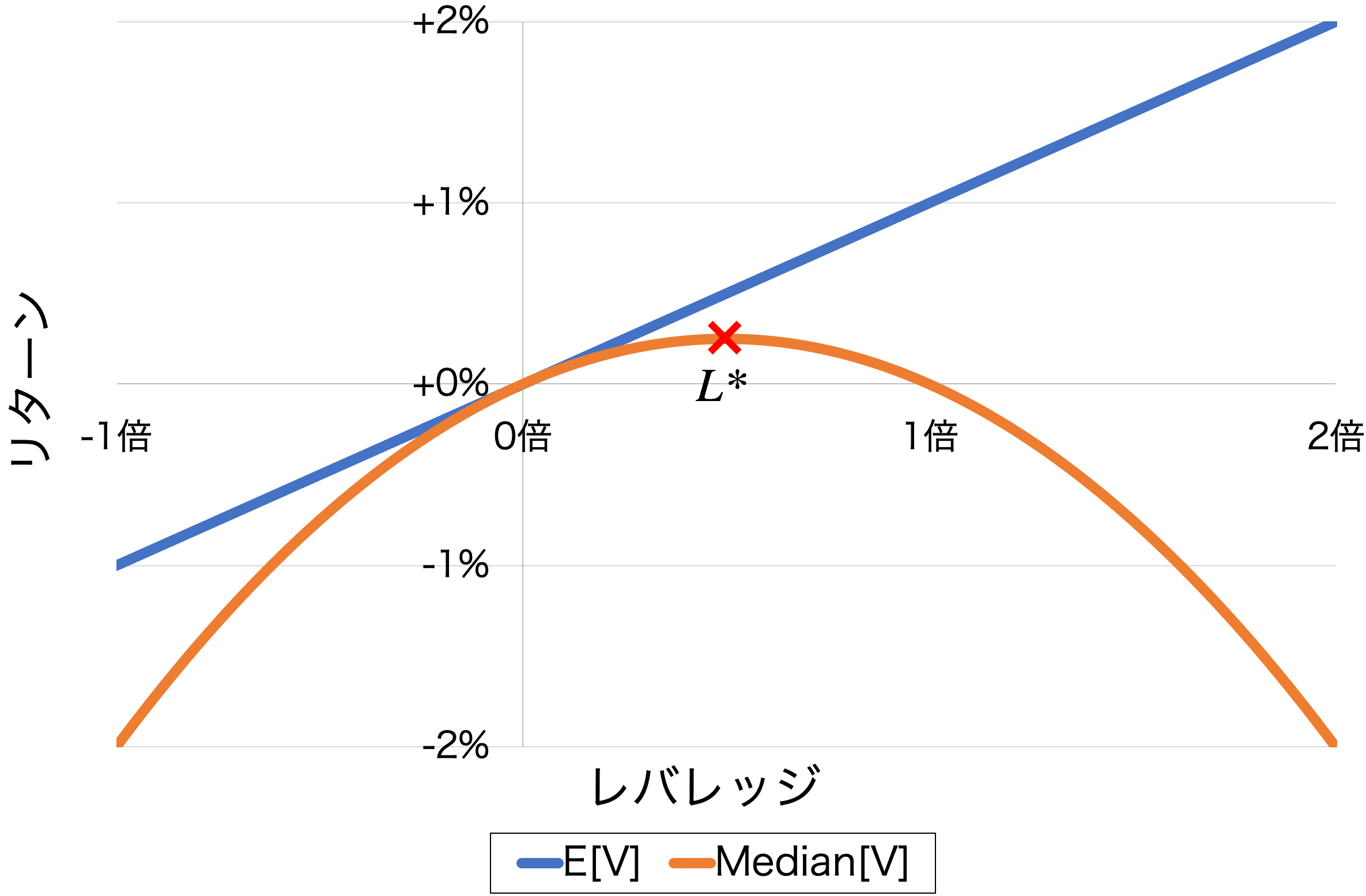
Figure 1.2.3: Relationship between leverage and return for the expected value and the median
From the figure above we see that the more leverage is applied, the more the median return diverges from the expected return, and we thus come to observe the decay of leveraged products.

1.2.4. Why We Use a Logarithmic Utility Function

As shown in Section 1.2.3, applying infinite leverage decreases the return in many cases, so we consider that each financial instrument has some optimal leverage. We therefore compute the optimal leverage L^* from the expected value {\rm E}[・], the Sharpe ratio {\rm SR}[・], and so on.
If we use the risk-neutral utility function U(x)=x, the expected value and the Sharpe ratio become indeterminate as follows, so they cannot be used to compute the optimal leverage.
\[ \displaystyle\arg\max_L[{\rm E}[V_t]] = \infty \]
\[ \begin{eqnarray} \displaystyle\arg\max_L[{\rm E}[{\rm SR}[V_t]]] & = & \arg\max_L\left[\frac{{\rm E}[V_0]\exp(Lμt)}{\sqrt{V_0^2L^2(σ^2t-μ^2t^2)}}\right] \\ & = & \begin{cases} \infty & (μ > 0)\\ -\infty & (μ < 0) \end{cases} \end{eqnarray} \]
If we use the logarithmic utility function U(x)={\rm ln}(x) as a risk-averse utility function, the expected value and the Sharpe ratio are obtained as follows.
\[ \displaystyle\arg\max_L[{\rm E}[\ln(V_t)]] = \frac{μ}{σ^2} \]
\[ \begin{eqnarray} \displaystyle\arg\max_L[{\rm E}[{\rm SR}[\ln(V_t)]]] & = & \arg\max_L\left[\frac{\left(Lμ - \frac{L^2σ^2}{2} \right)t}{\sqrt{L^2σ^2t}}\right] \\ & = & \frac{2μ}{σ^2} \end{eqnarray} \]
When a risk-averse utility function is used, as in equations (1.2.4c) and (1.2.4d), the optimal leverage can be determined as a value proportional to μ/σ^2. The constant of proportionality differs depending on the utility function but does not affect the calculation of portfolio composition. Considering the simplicity of the calculation and its good properties—such as coinciding with the optimal leverage of the median shown in Section 1.2.3 and coinciding with the answer derived from the Kelly criterionImos Financial Theory uses the logarithmic utility function U(x)={\rm ln}(x).
Among risk-averse utility functions that can form a consistent portfolio, a function for which the optimal leverage can be computed must satisfy that multiplying the leverage by N (multiplying μ by N and σ by N) multiplies it by 1/N, and that multiplying the unit time by T (multiplying μ by T and σ by \sqrt{T}) leaves it unchanged. Such a function is one proportional to μ/σ^2.

2. Portfolio Optimization

Imos Financial Theory uses a logarithmic utility function. We therefore explain how to compute the optimal portfolio under log utility.

3.1. Portfolio Optimization with Two Uncorrelated Assets

We consider the fluctuation when a portfolio is composed of two uncorrelated assets. From equation (1.2.1a), the fluctuation when a portfolio is composed using asset A and asset B can be expressed as follows.
\[ \displaystyle \begin{eqnarray} dV_t & = & \sum_{i \in \{{\rm A},\ {\rm B}\}} (L_iμ_idt + L_iσ_idB_{i,t}) \\ & = & \left( \sum_{i \in \{{\rm A},\ {\rm B}\}} L_iμ_i \right) dt + \sqrt{ \sum_{i \in \{{\rm A},\ {\rm B}\}} L_i^2σ_i^2 }dB_{t} \end{eqnarray} \]
Next, to optimize the portfolio, we evaluate it using the log expected utility. Using equation (1.1.3b), it is obtained as follows.
\[ {\rm E}[\ln(V_t)] = {\rm E}[\ln(V_0)] + \sum_{i \in \{{\rm A},\ {\rm B}\}} \left( L_iμ_i - \frac{(L_iσ_i)^2}{2} \right)t \]
Finding the leverages L_{\rm A},\ L_{\rm B} that maximize the above equation gives the following.
\[ \begin{aligned} L_i^* = \frac{μ_i}{σ_i^2} & & (i \in \{{\rm A},\ {\rm B}\}) \end{aligned} \]
From the above, we see that when newly trading an uncorrelated asset, its optimal leverage is determined regardless of whether one has already bought other financial instruments.

2.2. Portfolio Optimization with Multiple Correlated Assets

We consider the fluctuation when a portfolio vector L is composed of multiple correlated assets. Using the covariance matrix Σ, the fluctuation when the portfolio is composed can be expressed in the same form as equation (2.1a) as follows.
The covariance matrix Σ satisfies the following properties (reference: Covariance matrix - Wikipedia). \[ \begin{eqnarray} & \textbf{Σ} = E \left[ (\textbf{X}-\textrm{E}[\textbf{X}]) (\textbf{X}-\textrm{E}[\textbf{X}])^\top \right] & \\ & \Downarrow & \\ & \textbf{Σ} = \textrm{E}[\textbf{XX}^\top] - \textrm{E}[\textbf{X}]\textrm{E}[\textbf{X}]^\top & \end{eqnarray} \] Next, we define a matrix M that can express the correlations among the elements of the Brownian motion vector B_t using a Brownian motion B_{\rm I, t} whose elements are independent, as follows. \[ d\textbf{B}_t = \textbf{M} d\textbf{B}_{\rm I, t} \] From the two equations above, the matrix M can be expressed using the covariance matrix Σ as follows. \[ \begin{eqnarray} \textbf{Σ} & = & \textrm{E}[(\textbf{σ}^\top d\textbf{B}_t)(\textbf{σ}^\top d\textbf{B}_t)^\top] \\ & = & \textrm{E}[\textbf{σ}^\top \textbf{M} d\textbf{B}_{\textrm{I}, t} d\textbf{B}_{\textrm{I}, t}^\top \textbf{M}^\top \textbf{σ}] \\ & = & \textbf{σ}^\top \textbf{M} \textbf{M}^\top \textbf{σ} \end{eqnarray} \] From this, the variance of the assets V_t is obtained as follows. \[ \begin{eqnarray} \mathrm{Var}((\textbf{L} \circ \textbf{σ})^\top d\textbf{B}_t) & = & \textrm{E}[(\textbf{L} \circ \textbf{σ})^\top d\textbf{B}_t d\textbf{B}_t^\top (\textbf{L} \circ \textbf{σ})] \\ & = & \textbf{L}^\top (\textbf{σ}^\top \textbf{M} (\textrm{E}[d\textbf{B}_{\textrm{I}, t} d\textbf{B}_{\textrm{I}, t}^\top]) \textbf{M}^\top \textbf{σ}) \textbf{L} \\ & = & \textbf{L}^\top \textbf{Σ} \textbf{L} \end{eqnarray} \]
\[ \begin{eqnarray} dV_t & = & \textbf{μ}^\top\textbf{L} + \textbf{σ}d\textbf{B}_t\\ & = & \textbf{μ}^\top \textbf{L} + \sqrt{\textbf{L}^\top \textbf{Σ} \textbf{L}}dB_t \end{eqnarray} \]
Next, to optimize the portfolio, we evaluate it using the log expected utility. Using equation (1.1.3b), it is obtained as follows.
\[ {\rm E}[\ln(V_t)] = {\rm E}[\ln(V_0)] + \textbf{L}^\top \textbf{μ} - \frac{\textbf{L}^\top \textbf{Σ} \textbf{L}}{2} \]
Finding the portfolio L^* that maximizes the above equation gives the following.
The optimal portfolio L^* can be defined, from equation (2.2b), as the portfolio L that maximizes the following expression. \[ \textbf{L}^* = \arg\max_\textbf{L}\left( \textbf{μ}^\top \textbf{L} - \frac{\textbf{L}^\top \textbf{Σ} \textbf{L}}{2} \right) \] Since the covariance matrix is a non-negative matrix, the above is an upward-convex quadratic function, and it is maximized when the derivative inside the argmax on the right-hand side becomes the zero vector. Differentiating the expression inside the argmax with respect to L gives the following. \[ \begin{eqnarray} 0 & = & \frac{\partial}{\partial L} \left( μ^\top L - \frac{L^\top Σ L}{2} \right) \\ & = & μ - Σ L \end{eqnarray} \] Therefore, the optimal portfolio L^* is obtained as follows. \[ L^* = Σ^{-1} μ \]
\[ \begin{eqnarray} \textbf{L}^* & = & \arg\max_\textbf{L}\left( \textbf{μ}^\top \textbf{L} - \frac{\textbf{L}^\top \textbf{Σ} \textbf{L}}{2} \right) \\ & = & \textbf{Σ}^{-1} \textbf{μ} \end{eqnarray} \]
From the above, we see that when the fluctuations of the assets are linearly independent (when the inverse of the covariance matrix exists), the optimal leverage for multiple correlated assets is determined.

3. Fluctuation Model of Foreign Exchange

In Imos Financial Theory, we treat foreign exchange as an especially important financial instrument, because it has very high liquidity and fluctuates in a very ideal manner.

3.1. Fluctuation Model of Foreign Exchange

Because the fluctuation between currencies with very large markets—especially the dollar, euro, and yen—is ideal, the fluctuation over an infinitesimal time Δt, after canceling out the interest-rate differential, can be expressed as follows.
\[ \begin{eqnarray} S_{t+Δt} & = & \begin{cases} S_t (1 + σ\sqrt{Δt}) & \cdots & 50\% \\ S_t \frac{1}{1 + σ\sqrt{Δt}} & \cdots & 50\% \\ \end{cases} \end{eqnarray} \]
Consider two currencies A and B with sufficiently large real demand and high liquidity. Suppose people in each country buy the other currency and place an OCO order that takes profit when it becomes \exp(d) times or cuts loss when it becomes \exp(-d) times.
  • When currency A becomes \exp(d) times currency B, the order of people in country A becomes \exp(d) times and takes profit, while the order of people in country B becomes \exp(-d) times and cuts loss.
  • When currency A becomes \exp(-d) times currency B, the order of people in country A becomes \exp(-d) times and cuts loss, while the order of people in country B becomes \exp(d) times and takes profit.
If either the former or the latter had a higher probability, the fluctuations of currency A and currency B would no longer be commutative, which is a contradiction; therefore the two fluctuations are considered to be identical. From this, foreign-exchange fluctuation can be expressed by equation (1.1.1) in the state where r=0.
Transforming this into the form of equation (1.1.1b) gives the following.
\[ \begin{eqnarray} S_{t+Δt} & = & \begin{cases} S_t (1 + \frac{σ^2}{2}Δt + σ\sqrt{Δt}) & \cdots & 50\% \\ S_t (1 + \frac{σ^2}{2}Δt - σ\sqrt{Δt}) & \cdots & 50\% \\ \end{cases} \end{eqnarray} \]
From this, the fluctuation of foreign exchange can be expressed by the price-fluctuation model of financial instruments described in Chapter 1 with the expected return set to μ=σ^2/2 (the fact that the expected return is not 0 is known as Siegel's paradox). Computing the expected values under each utility function at this time using equations (1.2.2a) and (1.2.2b) gives the following, and the optimal leverage under the linear utility function is L^*=∞, while the optimal leverage under the logarithmic utility function is L^*=1/2.
\[ {\rm E}[V_t] = {\rm E}[V_0]\exp(\frac{1}{2}Lσ^2t) \]
\[ {\rm E}[\ln(V_t)] = {\rm E}[\ln(V_0)]+\frac{1}{2}L(1-L)σ^2t \]

3.2. Introducing the True Value

If we assume that there exists something called the "true value" and that each currency fluctuates with expected return μ=0 relative to the true value, the behavior becomes easier to understand when three or more currencies exist or when currencies with different volatilities exist. We therefore introduce that model.

3.2.1. Fluctuation of a Currency Relative to the True Value

The fluctuation of the asset value V_{{\rm true}, t} relative to the true value, when currency A with volatility σ is held at leverage L, is obtained as follows by substituting into equation (1.2.2b), from the assumption in Section 3.2 that it fluctuates with expected return μ=0.
\[ \textrm{E}[d\ln(V_{{\rm true}, t})] = -\frac{L^2σ^2}{2}dt \]

3.2.2. Three or More Currencies

Suppose there is a domestic currency S_t and N foreign currencies, each fluctuating independently with volatility σ relative to the true value. When each foreign currency is held at leverage L, the leverage of the domestic currency becomes 1-NL, so the asset value V_t relative to the domestic currency is obtained as follows using equation (3.2.1a).
\[ \begin{eqnarray} \textrm{E}[d\ln(V_t)] & = & \textrm{E}\left[ d\ln\left( \frac{V_{{\rm true}, t}}{S_{{\rm true}, t}} \right) \right]\\ & = & \textrm{E}[d\ln(V_{{\rm true}, t})] -\textrm{E}[d\ln(S_{{\rm true}, t})] \\ & = & -\frac{(1-NL)^2σ^2}{2}dt -\frac{NL^2σ^2}{2}dt +\frac{σ^2}{2}dt \\ & = & (1-(1-NL)^2-NL^2)\frac{σ^2}{2}dt \end{eqnarray} \]
The leverage L^* that maximizes the above equation is obtained as follows.
\[ \begin{eqnarray} L^* & = & \arg\max_{L}(1-(1-NL)^2-NL^2) \\ & = & \arg\max_{L}(-(N^2+N)L^2+2NL) \\ & = & \frac{1}{N+1} \end{eqnarray} \]
From the above equation, holding each currency equally, including the domestic currency, is the optimal portfolio that maximizes the logarithmic utility function of the asset value V_t relative to the domestic currency.

3.2.3. Currencies with Different Volatilities

Up to this point we assumed that all currencies have the same volatility. We now compute the optimal portfolio when currencies with different volatilities exist.
There is a domestic currency with volatility σ_{\rm self} relative to the true value, and a group of foreign currencies with a volatility vector σ. When the foreign currencies are held with a leverage vector L, the asset value V_t relative to the domestic currency is obtained as follows, similarly to equation (3.2.2a).
\[ \begin{eqnarray} \textrm{E}[d\ln(V_t)] & = & -\frac{(1-\displaystyle\sum_{i} \textbf{L}_i)^2σ_\textrm{self}^2}{2}dt -\frac{\displaystyle\sum_i \textbf{L}_i^2 \textbf{σ}_i^2}{2}dt +\frac{σ_\textrm{self}^2}{2}dt \end{eqnarray} \]
The optimal portfolio L^* that maximizes the above equation is obtained as follows.
Specifically, since the above equation is an upward-convex function, we see that it suffices to find the leverage vector L for which the partial derivative is 0. Taking the partial derivative of the above equation gives the following. \[ \begin{eqnarray} 0 & = & \frac{\partial}{\partial\textbf{L}_j}\textrm{E}[d\ln(V_t)] \\ & = & \left( 1 - \left( \displaystyle\sum_{i} \textbf{L}_i \right) \right) σ_\textrm{self}^2 - \textbf{L}_j \textbf{σ}_j^2 \end{eqnarray} \tag{3.2.3i} \] Transforming the above equation gives the following equation. \[ \textbf{L}_j=\frac{ \left( 1 - \left( \displaystyle\sum_{i} \textbf{L}_i \right) \right) σ_\textrm{self}^2 }{\textbf{σ}_j^2} \tag{3.2.3j} \] To expand the summation in the above equation, computing \sum_i L_i using the above equation gives the following. \[ \begin{eqnarray} \sum_i{\textbf{L}_i} & = & \left( 1 - \left( \displaystyle\sum_{i} \textbf{L}_i \right) \right) σ_\textrm{self}^2 \sum_i\frac{1}{\textbf{σ}_i^2} \\ & = & 1-\frac{1}{1+\displaystyle\sum_i\frac{σ_\textrm{self}^2}{\textbf{σ}_i^2}} \end{eqnarray} \tag{3.2.3k} \] Substituting the above equation into equation (3.2.3j), the optimal portfolio L^* is obtained as follows.
\[ \textbf{L}_j^*=\frac{1}{\displaystyle\frac{1}{σ_\textrm{self}^2}+\sum_i\frac{1}{\textbf{σ}_i^2}}\frac{1}{\textbf{σ}_j^2} \]
When currencies with different volatilities relative to the true value exist, we see that it is good to invest in proportion to the reciprocal of the volatility. From this, we also see that the conclusions of Section 3.1 and Section 3.2.2 hold only for currency pairs with the same variance relative to the true value.

4. Conclusion

  • As shown in Section 1.1.2, the price of a financial instrument that can be expressed using the Black–Scholes equation can be represented by a log-normal distribution.
  • As shown in Section 1.2.3, applying high leverage greatly reduces the median return.
  • As shown in Section 1.2.4, Imos Financial Theory uses the logarithmic utility function U(x)={\rm ln}(x). This coincides with optimizing so as to maximize the median of the price of a financial instrument that follows a log-normal distribution.
  • As shown in Section 1.2.4, the optimal leverage L^* that maximizes the median is obtained using the price S of the financial instrument as follows.
\[ L^* = \frac{μ}{σ^2} = \frac{\ln({\rm E}[S_t])-\ln(S_0)}{{\rm Var}[{\rm ln}(S_t)]} \]
  • As shown in Section 2.1, the optimal portfolio of multiple independently fluctuating assets coincides with the optimal leverage of each individual asset.
  • As shown in Section 2.2, the optimal portfolio of multiple correlated assets is obtained using the expected-return vector μ and the covariance matrix Σ as follows.
\[ L^* = Σ^{-1} μ \]
  • As shown in Section 3.1, in an environment where one can trade only a single foreign currency as stable as one's own, if one wishes to maximize the log expected utility of assets, this can be achieved by holding it at leverage 0.5 (half of the asset valuation in the foreign currency).