Bitcoin's Price Upside: A Long-Term Scenario Estimate
1. The range of prices through 2060
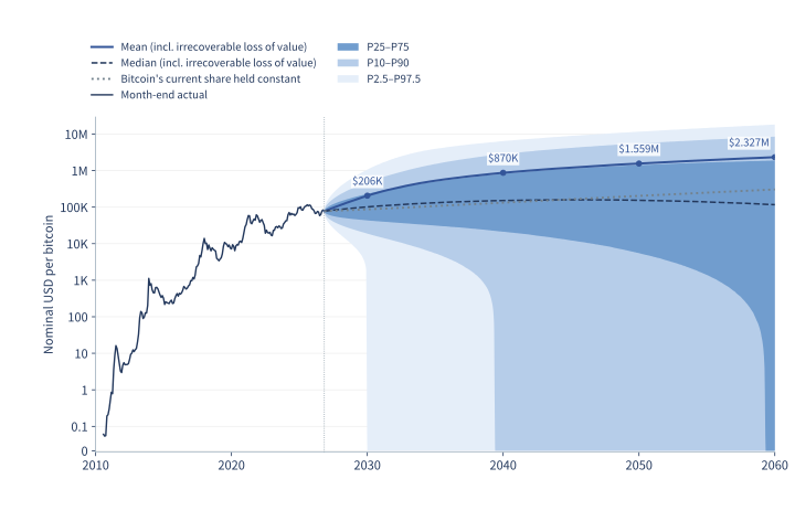
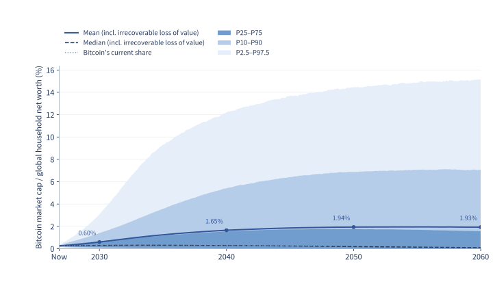
| Start of year | P10 | Median | Mean | P90 |
|---|---|---|---|---|
| 2030 | 19 | 101 | 206 | 483 |
| 2040 | 0 | 151 | 870 | 2,852 |
| 2050 | 0 | 154 | 1,559 | 5,534 |
| 2060 | 0 | 117 | 2,327 | 8,522 |
Inflation adjustment and price history
My cutoff for prices, supply, investment horizons, and loss probabilities is 00:00 UTC on November 1, 2026. The last daily price available was the October 31 Coin Metrics close of $77,401.02[10, 1]. All the statistics and surveys I use were published before the cutoff. The price history records give the observations and selection criteria. Each dataset lists the period it covers and its publication and access dates.
To express a nominal price in September 2026 dollars, I divide it by the ratio of the US Consumer Price Index at that date to its September 2026 level of 336.940. I use the all-items Consumer Price Index for All Urban Consumers (CPI-U), before seasonal adjustment[8, 9]. The same index converts world wealth and equity values. The portfolio simulation in §5 allows inflation to vary and uses each path's own price index to calculate final purchasing power.
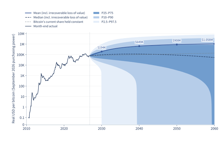
The historical line uses 196 UTC month-end observations from the Coin Metrics daily
PriceUSD series, July 2010 through October 2026[10, 1]. For the missing October 2025 CPI, I use the geometric mean of the adjacent months. For October 2026, I carry forward September's index, the latest available at the cutoff[11]. The Coin Metrics price history used in these charts is licensed under CC BY-NC 4.0[12].
- [8] U.S. Bureau of Labor Statistics, "Consumer Price Index — September 2026," 2026.
- [9] U.S. Bureau of Labor Statistics, "Consumer Price Index for All Urban Consumers: All Items in U.S. City Average [CPIAUCNS]," FRED, Federal Reserve Bank of St. Louis, 2026.
- [10] Coin Metrics, "USD Denominated Closing Price (PriceUSD)," 2026.
- [1] Coin Metrics, "Free Coin Metrics Data Archives," 2026.
- [11] U.S. Bureau of Labor Statistics, "2025 Federal Government Shutdown Impact on the Consumer Price Index," 2026.
- [12] Creative Commons, "Attribution-NonCommercial 4.0 International (CC BY-NC 4.0)," 2013.
2. World wealth as a benchmark
2.1. A price benchmark at Bitcoin's starting share
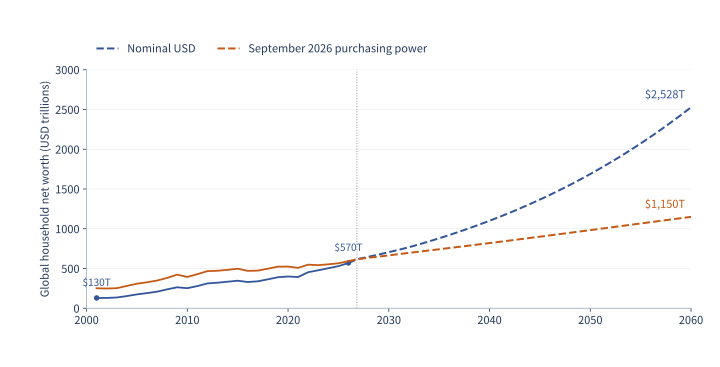
Historical wealth, future growth, and Bitcoin issuance
I use MGI's household wealth estimates for 2000, 2024, and 2025. For years between them, I interpolate the logarithm of the wealth-to-GDP ratio, convert it back to a ratio, and multiply by the IMF's nominal world GDP. For monthly values I interpolate log wealth with a cubic curve that preserves the direction of movement between observations.
Through 2031 I use the IMF forecasts for GDP and US consumer prices. After that I assume real world growth slows to 2.1% in 2040, 1.8% in 2050, and 1.5% in 2060, with long-run US inflation at 2.5%. The gap between the logarithm of the wealth-to-GDP ratio and its target, \(\log(4.5)\), halves every 15 years. The price forecast fixes nominal wealth and inflation along these paths, without additional shocks from recessions or exchange rates. The portfolio model allows inflation and short-term interest rates to fluctuate.
The Organisation for Economic Co-operation and Development projects in its 2025 outlook that slower population and productivity growth will reduce potential world growth to about 2.1% in the early 2040s and 1.3% in the second half of the century[13]. I chose the 2050 and 2060 rates to extend that slowdown smoothly. Actual world GDP in dollars also depends on exchange rates.
For long-run US inflation, the Congressional Budget Office projects 2.3%. In the Philadelphia Fed's third-quarter 2026 survey, forecasters expected inflation to average 2.6% over five years and 2.3% over ten[14, 15]. I extend my long-run assumption of 2.5% through 2060. My target wealth-to-GDP ratio of 4.5 falls between the historical ratios of about 3.8 in 2000 and 4.8 in 2025[2, 3]. MGI documents a period when asset revaluations outpaced economic growth[16]. The target and the 15-year adjustment half-life express my assumption that the two eventually grow at similar rates.
I project issuance from the April 20, 2024 halving using the block subsidy schedule and an average of ten minutes per block[17]. Market capitalization counts every coin issued, including coins whose owners have lost access to them.
- [13] OECD, "OECD Global Long-Run Economic Scenarios: 2025 Update," 2025.
- [3] International Monetary Fund, "World Economic Outlook Database, October 2026," 2026.
- [14] Congressional Budget Office, "The Budget and Economic Outlook: 2026 to 2036," 2026.
- [15] Federal Reserve Bank of Philadelphia, "Third Quarter 2026 Survey of Professional Forecasters," 2026.
- [2] McKinsey Global Institute, "The Global Balance Sheet 2026: Imbalance and Divergence," 2026.
- [16] McKinsey Global Institute, "Out of Balance: What’s Next for Growth, Wealth, and Debt?," 2025.
- [17] Bitcoin Core developers, "Bitcoin Core: GetBlockSubsidy," 2026.
2.2. Gold and Bitcoin relative to household wealth
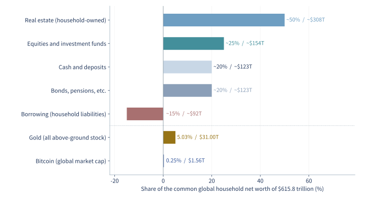
The denominator in the market-size comparison
MGI estimates household net worth at $570 trillion in 2025, worldwide net worth across all sectors at about $600 trillion, and gross assets across all sectors at $1,790 trillion[2]. Gross assets count financial claims across sectors. A household deposit, for example, is an asset for the household and a liability for the bank.
Gold and Bitcoin market values include holdings outside the household sector. Gold includes jewelry and central bank reserves, and I count gold held in exchange-traded funds (ETFs) once, as part of the underlying metal. A market worth 5% of household net worth need not make up 5% of household portfolios.
- [2] McKinsey Global Institute, "The Global Balance Sheet 2026: Imbalance and Divergence," 2026.
2.3. Market growth and shareholder returns
From total return to equity market capitalization
The J.P. Morgan and Vanguard outlooks in §5.1 give a nominal compound total return of about 6.7% per year for global equities when averaged on a log scale. Write this rate as \(c_E\), its logarithmic equivalent as \(g_E=\log(1+c_E)\), and the annualized volatility from the ten-year sample as \(\sigma_E\). In the diffusion model, the expected value after \(t\) years per dollar invested, with dividends reinvested, is \(T_E(t)=\exp\{(g_E+\sigma_E^2/2)t\}\).
Write total equity market capitalization as \(M_E=s_EW\), where \(s_E\) is its share of world wealth \(W\). Over a short interval, the expected shareholder return is approximately \(\mu_E\simeq g_W+g_{s_E}+d-n\). Wealth growth \(g_W\) and growth in the equity share \(g_{s_E}\) increase market value. Dividends add shareholder income at annual yield \(d\), while positive net issuance \(n\) (new issues less buybacks, as a fraction of market value) spreads that value over more shares[18, 19].
With each series starting at 1, removing reinvested dividends gives the expected price index \(P_E(t)\). Adding net issuance gives the expected market capitalization \(C_E(t)\). Dividing by the growth of wealth then gives the change in the equity share.
\[
P_E(t)=T_E(t)e^{-dt},\qquad
C_E(t)=P_E(t)e^{nt},\qquad
\frac{E[s_E(t)]}{s_E(0)}=\frac{C_E(t)}{W_t/W_0}.
\]
I assume a 2% dividend yield, between the lower US yields and the higher yields in several non-US markets in the institutional outlook[20]. I assume 0.5% annual net issuance. MSCI documents buybacks in developed markets and issuance in emerging markets, and J.P. Morgan expects new listings and stock-based compensation to grow. These two rates decompose the forecast total return, which already includes dividends.On the wealth path in §2.1, the equity market's expected share of world wealth rises to about 1.82 times its starting value by January 2060.
| Item | Start of 2030 | Start of 2040 | Start of 2060 |
|---|---|---|---|
| Global household net worth | 1.15 | 1.79 | 4.11 |
| Bitcoin price, current share held constant | 1.12 | 1.72 | 3.93 |
| Equity price index, expected value | 1.19 | 2.08 | 6.32 |
| Equity index including dividends, expected value | 1.27 | 2.71 | 12.27 |
| Intermediate-term US Treasuries including interest, expected value | 1.16 | 1.88 | 4.93 |
| Treasury bills including interest, expected value | 1.12 | 1.62 | 3.37 |
- [18] Gupta, Rohit, "Every Share Counts: The Impact of Buybacks on Markets," 2025.
- [19] MSCI, "How Is an Index Constructed?," 2026.
- [20] J.P. Morgan Asset Management, "2027 Long-Term Capital Market Assumptions," 2026.
3. Estimating Bitcoin's future share of world wealth
\[\boxed{P_t=s_tW_t/Q_t}\]
I use the same wealth projection and issuance schedule in all three valuation methods. What varies across price paths is Bitcoin's share, \(s_t\). A million-dollar bitcoin in January 2060 would put the market value of nearly 21 million coins at about $21 trillion. That would require about 0.83% of the projected $2.53 quadrillion in household net worth, up from 0.25% at the start.
3.1. A trend fitted to Bitcoin's market share
The fitted slowdown and the lower end of the historical distribution
A linear fit to the logarithm of Bitcoin's age makes the slope of the transformed market share fall in proportion to the reciprocal of age. I use a power transformation of age that includes the logarithm as a special case. This lets the last 120 monthly observations determine the rate of slowdown[21].
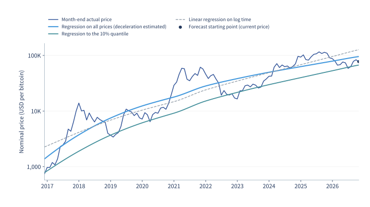
I also fit the conditional 10th percentile and median using all 120 observations in each quantile regression[22]. The 10th-percentile curve shows a slowdown too. The price forecast uses the least-squares fit.
The trend in the log odds of Bitcoin's share
Let \(X=\log\{s/(1-s)\}\) be the log odds of the share, \(A\) Bitcoin's age in years since January 3, 2009, and \(A_\star\) its age at the end of the sample. I fit
\[
X(A)=\alpha+bB_p(A/A_\star)+e,\qquad
B_p(z)=\begin{cases}(z^p-1)/p & p\ne0,\\ \log z & p=0.\end{cases}
\]
Here \(\alpha\) sets the level, \(b\) the slope at the reference age in scaled time, \(p\) the curvature, and \(e\) is the residual. At \(p=0\) the trend is linear in log age. I restrict \(p\le1\), so a positive slope stays constant or declines. The fit gives \(b\simeq2.404\) and \(p\simeq-1.525\) using the wealth series from §2.1. Resampling residuals in six-month blocks gives 8,192 slope–shape pairs. Extending the search for \(p\) from −8 down to −12 leaves the fit unchanged, and none of the ten-year resamples hits the original lower bound.
The slope with respect to age is
\[
\frac{dX}{dA}=\frac{b}{A_\star}(A/A_\star)^{p-1}
\]
Starting from the observed \(X_0\) at age \(A_0\), I project the trend as \(X_0+\widehat X(A_0+t)-\widehat X(A_0)\), where \(\widehat X\) is the fitted curve and \(t\) is the forecast horizon in years. Its starting slope is 0.135 per year, compared with 0.253 for the log-age fit. At Bitcoin's small initial share these correspond to annual log growth in the share of about 13.5% and 25.3%. To obtain an arithmetic mean price, I convert individual simulated shares to prices and then average them. Converting the center of a log-scale forecast gives a different quantity[23].
Historical forecast errors and market volatility
At quarterly dates from June 2018 onward, I refit each curve using up to the preceding 120 monthly observations and compare its forecast with the subsequent change in \(X\)[23]. The historical household wealth series is reconstructed as in §2.1. Estimating the slowdown reduced the root-mean-square error in log odds from 0.735 to 0.718 over 30 one-year forecasts and from 0.897 to 0.886 over 26 two-year forecasts.
The gains are small and the forecast windows overlap. The fits and forecast errors cover horizons of one and two years. The projection to 2060 is a much longer extrapolation.
To estimate ordinary market volatility, I subtract the fitted change in \(X\) from each of the last 120 monthly changes and divide each difference by the square root of that month's length in years. Their standard deviation gives a starting annualized volatility \(\sigma_0\simeq0.6855\). J.P. Morgan's 2027 assumptions give a long-run reference value of 55%[20]. I connect the two with \(\sigma(t)=0.55+(\sigma_0-0.55)e^{-t/15}\).
I chose the 15-year time constant, so the gap to 55% halves in about 10.4 years. J.P. Morgan supplies the long-run risk assumption. The rate of convergence and its extrapolation through 2060 are mine. Section 3.3 compares alternative time constants.
The volatility estimates by period show how much the choice of window matters. Measured from daily price changes, annualized volatility was 67.4% over the last ten years, 50.7% over five, and 43.7% over one[1]. I use ten years of monthly residuals so the recent quiet period carries less weight. In §3.5 I shorten the window to 60 months for the trend and, separately, for volatility. I also test the simpler trend fitted to the logarithm of Bitcoin's age.
- [21] G. E. P. Box, D. R. Cox, "An Analysis of Transformations," 1964.
- [22] Roger Koenker, Gilbert Bassett Jr., "Regression Quantiles," 1978.
- [23] Rob J. Hyndman, George Athanasopoulos, "Forecasting: Principles and Practice, Third Edition: The Forecaster's Toolbox," 2021.
- [20] J.P. Morgan Asset Management, "2027 Long-Term Capital Market Assumptions," 2026.
- [1] Coin Metrics, "Free Coin Metrics Data Archives," 2026.
3.2. Demand by type of holder
Investable assets and flows into and out of Bitcoin
I estimate gross household financial assets at $400 trillion, about 65% of starting household net worth using MGI's rounded breakdown[2]. Allianz puts pension and insurance claims at 24.8% of household financial assets. To split them, I use the Financial Stability Board's $44.1 trillion in pension assets and $38.9 trillion in insurance assets as relative weights[24, 25]. This approximates the breakdown of household claims from institutions' balance sheets. Counting exchange-traded funds (ETFs) or asset managers again would duplicate assets already held for beneficiaries.
For corporate cash I use Damodaran's $11.4 trillion for listed nonfinancial companies in July 2025 as a proxy for year-end 2025, then scale it by household wealth growth up to November 2026[26]. IE University and ICEX-Invest in Spain report $15.1 trillion in sovereign wealth funds as of April 2026, and the IMF reports $13.22 trillion in foreign exchange reserves for the second quarter[27, 28]. Some corporate cash is already reflected in equities owned by households. I deduct 50% of corporate cash in the central case and let the deduction vary uniformly from 0% to 100% to allow for the unknown overlap.
For sector \(i\), let \(F_i\) be its investable assets excluding bitcoin, \(a_i\) the fraction of those assets owned by adopters, and \(w_i\) the fraction of an adopter's total investable assets allocated to bitcoin. Adopters own \(F_i a_i\) in other assets, so their desired bitcoin holdings are \(F_i a_iw_i/(1-w_i)\). The basic adoption equation is \(a_i'=\lambda_i(1-a_i)-\mu_i a_i\). The annual adoption rate \(\lambda_i\) applies to nonadopters' assets and the exit rate \(\mu_i\) to adopters' assets. The target allocation reflects ordinary volatility and the losses holders can tolerate. Section 3.5 adds the cost of unusually concentrated positions.
Adoption and exit rates
The share of US adults who had bought or held crypto assets as an investment in the previous year was 11%, 8%, 7%, 7%, and 9% in successive surveys from 2021 to 2025[29]. UK crypto ownership fell from 12% in 2024 to 8% in 2025. In Canada, Bitcoin ownership fell from about 13% in 2021 to 10% in 2023[30, 31]. These reversals motivate allowing holders to exit. The surveys count people, whereas the model needs the value of assets entering and leaving.
I give equal weight to stalled, gradual, and rapid adoption. In the gradual case, the rates vary around the values below. The adoption share measures how much of the sector's asset base belongs to adopters.
| Sector | Adoption share at start | Annual adoption rate | Annual exit rate | Baseline Bitcoin share of adopters' portfolios |
|---|---|---|---|---|
| Newly adopting households | 0% | 2.0% | 5.0% | 1.0% |
| Pensions | 0.5% | 1.5% | 4.0% | 0.4% |
| Insurers | 2.0% | 0.6% | 4.0% | 0.075% |
| Corporate cash | 1.0% | 1.8% | 8.0% | 2.0% |
| Sovereign wealth funds | 4.0% | 1.5% | 4.0% | 0.5% |
| Central banks | 0% | 0.1% | 5.0% | 0.2% |
For households, a 2% adoption rate and a 5% exit rate balance when adopters own \(2/(2+5)\simeq29\%\) of the asset base. The adjustment has a time constant of about 14 years. I vary the rates by sector to reflect pension and sovereign funds' long horizons, investment constraints on insurers and central banks, and companies' need for working capital.
I assign holdings left unexplained by the sector estimates to a separate group of existing holders, with a central exit rate of 1.5% per year. When calculating new household demand, I exclude assets that remain in this group.
In Deloitte's survey of finance chiefs at large companies, 23% intended to use crypto assets for payments or investment within two years[32]. The EY/Coinbase survey covers institutions that already invest or plan to do so[33]. These surveys describe intentions among particular respondents. I use judgment to turn that evidence and sector constraints into the starting shares and transition rates.
How much adopters hold
A sector's overall exposure combines participation and position size. For the position sizes below, I use holdings reported by individual adopters and comparisons with institutional risk budgets.
UBS reports a typical crypto allocation of about 1% among family offices that hold crypto assets. BlackRock illustrates a 1–2% Bitcoin allocation based on its contribution to portfolio risk[34, 35]. I use 1% for newly adopting households, extrapolating from the wealthy families served by family offices and from a model portfolio.
At the end of 2024, the State of Wisconsin Investment Board held about $322 million in Bitcoin ETFs, or about 0.20% of its more than $162 billion under management. The denominator includes the board's nonpension assets[36, 37]. I center pension adopters' allocations at 0.4%, between this example and BlackRock's illustrative 1–2%, and vary the estimate to allow for other funds' practices[35].
MassMutual's $100 million purchase was about 0.045% of its $224 billion general account, according to Conning[38]. Across EU insurers, including nonholders, the European Insurance and Occupational Pensions Authority reports crypto exposure of about 0.0068%. Most respondents in a Goldman Sachs insurance survey also held none[39, 40]. I use 0.075% for the allocation among adopters and a low participation rate for the industry as a whole.
Nexon invested less than 2% of its cash in bitcoin at the time of purchase[41]. Square's October 2020 and February 2021 purchases cost $220 million, about 5% of its $4.3 billion in cash, cash equivalents, restricted cash, and marketable debt securities at the end of March 2021[42]. The second comparison uses a balance measured after the purchases. I assume an allocation of 2% of corporate cash.
For sovereign wealth funds I use 0.5%. Mubadala's roughly $490 million in Bitcoin ETFs in June 2026 amounts to about 0.13% of its $385 billion under management at year-end 2025. Luxembourg's sovereign fund set a 1% crypto allocation[43, 44, 45]. The first comparison uses balances from different dates, and the second is a policy target.
The Czech National Bank decided against investing its foreign exchange reserves in bitcoin at the time and created a separate pilot portfolio[46]. The IMF reserve management guidelines prioritize liquidity and safety ahead of return[47]. I start formal central bank adoption at zero, assume slow entry, and allow future adopters to allocate 0.2%. The model accounts separately for governments retaining confiscated coins.
Risk budgets and uncertainty about existing holdings
I calibrate loss and volatility budgets from the baseline allocations, a 75% peak-to-trough decline, and the ten-year volatility estimate of 68.5%. Bitcoin's past large declines reached 70–80%[48]. For stalled, gradual, and rapid adoption respectively, I assume drawdowns of 85%, 70%, and 55%, paired with volatilities of 68.5%, 55%, and 44%. The last two volatility figures draw on J.P. Morgan's long-run assumption and Fidelity's second-quarter 2026 estimate of long-run realized volatility[20, 49]. Pairing wider adoption with milder declines is my scenario choice.
I assume that holders use, on average, two-thirds of their risk budget. The 1% allocation I assume for new household adopters is two-thirds of 1.5%, the midpoint of BlackRock's 1–2% example[34, 35]. I use the same average for other sectors, drawing utilization from \(\operatorname{Beta}(4,2)\). It allows partial use of the budget. A holding must be less than the whole portfolio, but I impose no fixed sector cap. In the gradual case, the loss holders can tolerate in a steep decline limits their positions even when volatility falls.
For existing holders whose sector is unknown, I infer the allocation needed to match the starting price. I assume that their share of household assets follows a triangular distribution with minimum 7%, mode 13%, and maximum 22%. Surveys place ownership near one person in ten. I widen the range when translating that headcount into wealth because assets are unevenly distributed and holders are hard to classify.
For coins that governments retain, I assume a triangular distribution from zero to 600,000, with a mode of 300,000. BitcoinTreasuries estimated government holdings at about 645,000 coins at the end of November 2025 from public information[50]. The US reserve has a retention policy[51]. How many of the reported coins governments will keep is uncertain. The model derives new purchases separately from central bank and sovereign fund budgets.
Across sectors, I vary adoption rates, exit rates, and holding budgets with log standard deviations of roughly 0.2–0.45. I allow for a common 6% error in asset amounts and a 4% sector-specific error, a pension share of 43–63% of pension and insurance assets combined, and a 0–6% allowance for incomplete coverage. These ranges reflect differences in survey dates, populations, and definitions. The parameter sources and assumptions document each choice.
With a log standard deviation of 0.45, the middle 80% of values spans about 0.56–1.78 times the median. At 0.20 it spans about 0.77–1.29 times the median. For budget utilization, the chosen beta distribution puts the middle 80% between 42% and 89%. The European Food Safety Authority and O'Hagan discuss how to distinguish observations from expert judgment and examine distribution shapes and dependencies[52, 53]. I chose these distributions myself, without a formal elicitation from experts.
Each sector's assets grow with real household net worth. At each date I divide total desired bitcoin holdings by world wealth in the same dollars, then compare that ratio with its starting value. Price expectations do not enter the sector holding budgets.
- [2] McKinsey Global Institute, "The Global Balance Sheet 2026: Imbalance and Divergence," 2026.
- [24] Allianz, "Global Wealth Report 2026: Financial Assets," 2026.
- [25] Financial Stability Board, "Global Monitoring Report on Non-Bank Financial Intermediation 2025," 2025.
- [26] Aswath Damodaran, "To Bitcoin or Not to Bitcoin: The Corporate Cash Question," 2025.
- [27] IE University, ICEX-Invest in Spain, "Sovereign Wealth Funds Surpass 15 Trillion in Assets," 2026.
- [28] International Monetary Fund, "COFER Data Brief, September 30, 2026," 2026.
- [29] Board of Governors of the Federal Reserve System, "Economic Well-Being of U.S. Households in 2025: Banking," 2026.
- [30] Financial Conduct Authority, "Cryptoassets Consumer Research 2025, Wave 6," 2025.
- [31] Bank of Canada, "Canadian Bitcoin Ownership in 2023: Key Takeaways," 2025.
- [32] Deloitte, "Q2 2025 CFO Signals: Corporate Crypto Adoption," 2025.
- [33] EY-Parthenon, Coinbase, "2026 Institutional Investor Digital Assets Survey," 2026.
- [34] UBS, "UBS Global Family Office Report 2026," 2026.
- [35] BlackRock Investment Institute, "Sizing Bitcoin in Portfolios," 2024.
- [36] State of Wisconsin Investment Board, "Form 13F Information Table for 2024 Q4," 2025.
- [37] State of Wisconsin Investment Board, "SWIB Fact Sheet: December 31, 2024," 2025.
- [38] Conning, "Crypto Comes into Focus," 2021.
- [39] European Insurance, Occupational Pensions Authority, "Technical Advice on Standard Formula Capital Requirements for Investments in Crypto-Assets," 2025.
- [40] Goldman Sachs Asset Management, "Global Insurance Survey 2026: Adaptation in Action," 2026.
- [41] NEXON, "Nexon Purchases 100 Million Dollars Worth of Bitcoin," 2021.
- [42] Square, "Form 10-Q for the Quarter Ended March 31, 2021," 2021.
- [43] Mubadala Investment Company, "Form 13F Information Table for 2026 Q2," 2026.
- [44] Mubadala Investment Company, "Strong Performance by UAE Portfolio Drives Mubadala Growth in 2025," 2026.
- [45] Ministère des Finances, Luxembourg, "Fonds souverain intergénérationnel du Luxembourg: Politique générale," 2025.
- [46] Czech National Bank, "Balancing Volatility and Returns in the Czech National Bank Foreign Exchange Portfolio: Update on Gold and Bitcoin," 2026.
- [47] International Monetary Fund, "Revised Guidelines for Foreign Exchange Reserve Management," 2013.
- [48] BlackRock, "Bitcoin Volatility Guide: Trends and Insights for Investors," 2025.
- [20] J.P. Morgan Asset Management, "2027 Long-Term Capital Market Assumptions," 2026.
- [49] Fidelity Digital Assets Research, "Signals Report Q2 2026," 2026.
- [50] BitcoinTreasuries.net, "November 2025 Corporate Adoption Report," 2025.
- [51] The White House, "Establishment of the Strategic Bitcoin Reserve and United States Digital Asset Stockpile," 2025.
- [52] EFSA Scientific Committee, "Guidance on Uncertainty Analysis in Scientific Assessments," 2018.
- [53] Anthony O'Hagan, "Expert Knowledge Elicitation: Subjective but Scientific," 2019.
3.3. Equilibrium between holding benefits and investment risk
The return a holder requires
Let \(w\) be Bitcoin's share of participants' investable assets and \(\mu_1(w,t)\) the real expected return they require \(t\) years from the start. The real short-term rate is \(r\), the cost of holding bitcoin is \(f\), the benefit coefficient is \(\eta\), and relative risk aversion is \(\gamma_i\). The hazard rate \(\lambda\) measures the instantaneous risk of permanent loss given survival. Bitcoin has expected volatility \(\sigma_{\rm e}\) in this calculation and return correlation \(\rho\) with equities. The equity Sharpe ratio \(S\) is expected excess return over the short-term rate divided by volatility. For small positions \(w\), I approximate the required return by
\[
\mu_1(w,t)=r+\rho\sigma_{\rm e} S+f-\eta/w
+\gamma_i\sigma_{\rm e}^2(1-\rho^2)w+\lambda(1+\gamma_iw)
\]
Equity returns, volatility, interest rates, and Bitcoin's correlation with equities use the assumptions and ten-year history in §5. I solve the equation under 20,000 sets of assumptions about participation, benefits, and risk. I set the required real return in 2200 equal to long-run real world wealth growth and integrate backward to the forecast origin. The volatility holders expect in this equation is distinct from the volatility used to simulate ordinary market shocks in §§3.5 and 5.
Transaction benefits, risk, and costs
In the model of Biais et al., future net transaction benefits support Bitcoin's price[54]. Cong et al. model how differences among users and network effects connect adoption and valuation in both directions[55]. These theories motivate assigning value to the services a holder obtains.
I choose a logarithmic benefit with marginal benefit \(\eta/w\). A small holding gives the owner the option to store and transfer value, and each additional unit adds less. Because the marginal benefit grows without bound as \(w\) approaches zero, a positive \(\eta\) implies some demand as long as Bitcoin survives. The benefit itself can also decline. Zimmerman models how speculation and limited settlement capacity can reduce the value of using the network[56].
| Parameter | Central value | Basis or interpretation |
|---|---|---|
| Initial annual volatility | 68.5% | Estimated from 120 monthly changes around the fitted trend. |
| Long-run annual volatility | 55% | J.P. Morgan's illustrative risk assumption. Fidelity reports 44% long-run realized volatility, and BlackRock documents a decline over time. |
| Volatility time constant | 15 years | Half the gap to long-run volatility closes in 10.4 years. |
| Relative risk aversion | 4 | Barro uses coefficients of 3 and 4 in a model of disaster risk. |
| Annual holding cost | 0.25% → 0.20% | The fees on the Bitcoin exchange-traded funds IBIT and BITB approximate custody and management costs. |
| Asset-weighted participation | 30% → 65% | Surveys distinguish investors who hold crypto assets from those considering a purchase. I use the headcounts to guide an assumption about wealth. |
| Participation time constant | 16 years | Half the gap to long-run participation closes in 11.1 years. |
| Long-run benefit multiple | Median 1 | Benefit relative to its starting value. Scenarios allow gains and declines. |
| Benefit time constant | 20 years | Half the gap to the long-run benefit multiple closes in 13.9 years. |
The volatility sources cover different periods. J.P. Morgan limits its 55% assumption to an illustrative matrix of a few assets because Bitcoin's correlations are unstable[20, 49, 48]. I vary volatility around that value along with participation and benefits. Relative risk aversion governs the amount of risk investors accept in Merton's model, and Barro uses values of 3 and 4 for disaster risk[7, 57]. I chose 4 as a comparable magnitude.
I use the funds' published fees as a proxy for holding costs. Self-custody costs, trading costs, and taxes fall outside that proxy[58, 59]. The participation path also enters the concentration calculation in §3.5. The short-term rate, equity Sharpe ratio, and correlation with bitcoin use the inputs in §5.1.
Calibration to the starting price
I infer \(\eta\) by matching the baseline valuation to the observed November 2026 price. Each scenario starts with a log valuation multiple of zero, so the model estimates how valuation changes from that common starting point.
Across the 20,000 sets of inputs, the middle 80% spans 19–43% for initial participation, 41–83% for long-run participation, 2.6–6.2 for risk aversion, and 0.38–2.63 for the long-run benefit multiple. These ranges express my uncertainty about applying the surveys and theories to future holders. The benefit multiple has a median of 1 and a mean of about 1.33 because its upper tail is long.
I also assume that greater participation tends to accompany lower volatility and larger benefits. In the draws, long-run participation has a correlation of −0.69 with long-run volatility and +0.33 with the benefit multiple. Network effects in Cong et al. could link adoption with benefits, while the congestion in Zimmerman's model could weaken that link[55, 56]. These correlations describe assumptions about future inputs. Section 5 estimates correlations between asset returns from historical data.
Sensitivity to timing and dependence
In Goldman Sachs family office surveys, crypto ownership rose from 16% in 2021 to 26% in 2023 and 33% in 2025[60]. Fitting an exponential approach to an assumed final 65% gives a time constant of 9.2 years. Varying just the final level from 50% to 80% gives 5.8–12.6 years, so this short series gives little leverage to estimate both the final level and the speed of adoption. I choose 16 years for the worldwide asset-weighted share because I assume slower adoption than these family office headcounts suggest.
| Baseline time constant | Halved | Doubled |
|---|---|---|
| Participation (16 years) | −7.5% | +1.6% |
| Volatility (15 years) | −3.4% | 0.0% |
| Benefit (20 years) | −0.5% | +0.6% |
For each of 1,024 matched parameter sets I divide the modified valuation multiple by its baseline counterpart, take the median of those ratios, and subtract 1. This isolates the equilibrium calculation before combining it with the other methods, market fluctuations, and permanent loss.
To test the dependence assumptions, I separately shuffled long-run participation and the benefit multiple across parameter sets, preserving each distribution. In four shuffles, the median January 2060 valuation multiple fell by 0.7–2.3%. Individual cases moved much more. The middle 80% of shuffled-to-original ratios spanned roughly 0.55–1.82.
The time-constant and dependence checks follow the uncertainty-analysis practice of testing both input ranges and how inputs co-vary[52, 53].
The terminal real return is 1.5%, the long-run real growth rate in §2.1. Moving the terminal year from 2200 to 2300 changed the January 2060 valuation multiple by at most 0.006% across 512 matched cases. Halving the long-run benefit multiple lowered the valuation multiple by a median 26%, and doubling it raised the valuation multiple by a median of 29%. The matched comparisons show how much more the equilibrium valuation depends on the assumed benefit than on the terminal date.
- [54] Biais, Bruno, Bisière, Christophe, Bouvard, Matthieu, Casamatta, Catherine, Menkveld, Albert J., "Equilibrium Bitcoin Pricing," The Journal of Finance 78(2), 967―1014, 2023.
- [55] Lin William Cong, Ye Li, Neng Wang, "Tokenomics: Dynamic Adoption and Valuation," 2021.
- [56] Peter Zimmerman, "Blockchain Structure and Cryptocurrency Prices," 2020.
- [20] J.P. Morgan Asset Management, "2027 Long-Term Capital Market Assumptions," 2026.
- [49] Fidelity Digital Assets Research, "Signals Report Q2 2026," 2026.
- [48] BlackRock, "Bitcoin Volatility Guide: Trends and Insights for Investors," 2025.
- [7] Merton, Robert C., "Lifetime Portfolio Selection under Uncertainty: The Continuous-Time Case," The Review of Economics and Statistics 51(3), 247―257, 1969.
- [57] Robert J. Barro, "Rare Disasters and Asset Markets in the Twentieth Century," 2006.
- [59] Bitwise, "Bitwise Bitcoin ETF: Sponsor Fee," 2026.
- [60] Goldman Sachs, "Adapting to the Terrain: Family Office Investment Insights," 2025.
- [52] EFSA Scientific Committee, "Guidance on Uncertainty Analysis in Scientific Assessments," 2018.
- [53] Anthony O'Hagan, "Expert Knowledge Elicitation: Subjective but Scientific," 2019.
3.4. Combining the three valuations
The quantities that enter the average
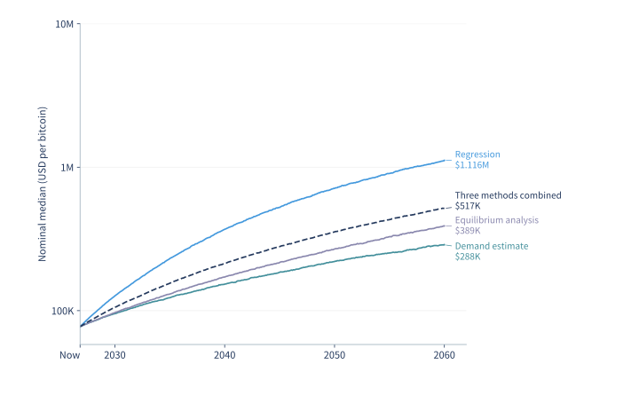
Forecast combination is an established approach when different models describe the same outcome[61]. I set each model's starting change to zero and average subsequent changes with weights of one-third. The regression supplies the change in the log odds \(X=\log\{s/(1-s)\}\). Sector demand supplies the log change in desired holdings relative to world wealth. For equilibrium demand, I multiply asset-weighted participation by \(w/(1-w)\), where \(w\) is the bitcoin weight in participants' portfolios, and take the change in the logarithm of that product.
I use the average as the change in \(X\) before the additional effects in §3.5. Treating the three transformed quantities as comparable is an assumption. I give the methods, and the three sector adoption scenarios, equal weight because I have little evidence for preferring one.
- [61] Allan Timmermann, "Forecast Combinations," Handbook of Economic Forecasting 1, 135―196, 2006.
3.5. Concentration costs and market volatility
The cost of a concentrated position
Let \(a_t\) be participants' investable assets divided by world wealth. Bitcoin's share of those participants' portfolios is \(w=s/a_t\). My central path is \(a_t=0.5\{0.65+(0.30-0.65)e^{-t/16}\}\). The factor 0.5 approximates investable assets using MGI's gross household financial assets of about 65% of net worth less liabilities of about 15%[2].
UBS and Goldman Sachs found that 24% and 33% of family offices, respectively, held crypto assets[34, 60]. I put starting participation at 30%. For the long run I choose 65%, between the 56% of Goldman Sachs respondents who already held crypto assets (33%) or expressed interest (23%), and the 74% in BNY's survey who held, had limited holdings, or were considering them[60, 62]. In Fidelity's 2022 survey, 42% of US institutional respondents held digital assets, compared with 67% in Europe and 69% in Asia[63]. Translating headcounts and intentions into a future share of global financial assets requires judgment.
At 50% investable wealth and 30% participation, Bitcoin's initial market value equals 1.68% of participants' investable assets. This is close to BlackRock's illustrative 1–2% allocation[35]. The 1.68% follows from the observed price and assumed participation, so it cannot independently validate adoption. I use the same participation path as in §3.3, with a 16-year time constant and an 11.1-year half-life.
I use the permanent-loss hazard rate \(\lambda_t\), relative risk aversion \(\gamma_c=4\) for concentration risk, and an annual yield \(y=3\%\) for income forgone on competing assets. The risk aversion follows the scale in §3.3[57]. I chose the 3% proxy between the 2% assumed equity dividend yield in §2.3 and the 3.7% long-run Treasury bill return in §5.1[20, 6]. Removing the first-order terms already represented in the individual methods leaves an extra cost of
\[
H_t(w)=\lambda_t\{(1-w)^{-\gamma_c}-1-\gamma_cw\}
+y\frac{w^2}{1-w}
\]
The first remaining terms are quadratic in \(w\). The extra cost is small for small positions and increases steeply as \(w\) approaches 1.
Write \(g_{\rm native}(t)\) for the annual rate of valuation change from §3.4 and \(X_t=\log\{s_t/(1-s_t)\}\) for the log odds of Bitcoin's share. I evolve \(X_t\) over the \(t\) years after the forecast origin according to
\[
dX_t=\left[g_{\rm native}(t)-\kappa\{H_t(s_t/a_t)-H_t(s_0/a_t)\}\right]dt
+\sigma(t)dB_t
\]
At each date, I subtract the cost the starting share \(s_0\) would incur with that same date's available wealth \(a_t\). The difference measures the cost attributable to the change in Bitcoin's share. I set \(\kappa=1\), so each extra percentage point of annual cost reduces the annual drift in \(X\) by the same amount. This is an assumed price response. I also test \(\kappa=0.5\), 4, and 0. The random term uses standard Brownian motion \(B_t\) and the volatility \(\sigma(t)\) in §3.1.
With a positive response, the model keeps \(s_t\lt a_t\), so Bitcoin's market value stays below participants' investable assets. In the zero-response comparison that concentration constraint also disappears. The parameter evidence records the basis for the response, investable share, risk aversion, competing yield, and volatility. I use the same random market shocks when comparing alternative assumptions.
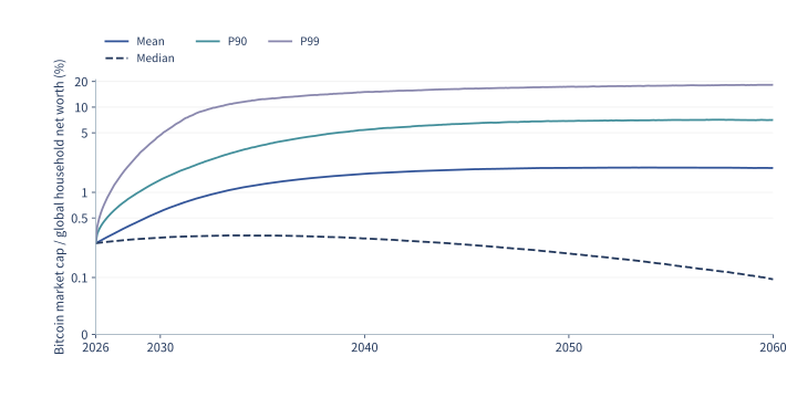
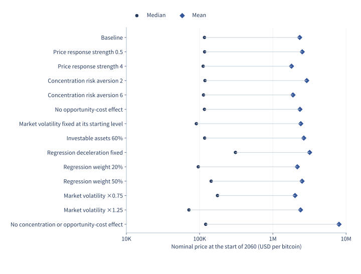
I split each month into two steps and solve a monotone equation for the share at the end of each step. Using four steps with the same random draws changed mean prices at the start of 2030, 2040, 2050, and 2060 by at most 0.23%. I also checked a different root solver and different random seeds. The additional sensitivity runs use 65,536 paths. The price model assumptions, numerical checks, and simulation code give the details.
4. The probability of permanent loss
4.1. The record of comparable crypto assets
Which losses the historical record can establish
I take the ten largest assets in CoinMarketCap's December 31, 2013 snapshot and follow the nine other than Bitcoin[64]. In pages archived between February and October 2026, four were untracked or marked as previews. I exclude NXT because Jelurida announced its migration to Ardor in February 2026[65]. For the three remaining candidates, the archived status establishes neither a 99% loss nor the impossibility of recovery. CoinMarketCap also stops tracking assets for lack of trading data or failure to meet listing criteria[66]. The nine-asset record gives each archive date. Changes between those dates and November 1 are unknown.
Of \(n\) comparison assets, let \(k\) be candidates for permanent loss and \(r\) the fraction of candidates that actually meet the definition. That gives an estimated historical loss fraction of \(p=(k/n)r\) over \(T\) years. Assuming a constant hazard rate for the group and a hazard rate \(c\) times as large for Bitcoin, its cumulative probability of loss over the next \(t\) years is
\[
q_{\rm ref}(t)=1-(1-p)^{ct/T}
\]
The central case uses \(k=3,n=9,r=0.50,c=0.25\), with \(T\) about 12.84 years. I count half the candidates as losses to allow for missing trading data and surviving claims, and set Bitcoin's hazard rate at one-quarter of the comparison group's. Cong et al. give a reason to expect network size to matter[55]. Budish points out that a larger economic prize can also make an attack more attractive[67]. Neither result determines the multiplier.
| Case | Candidates \(k\) | Fraction qualifying \(r\) | Hazard multiplier \(c\) | Loss probability |
|---|---|---|---|---|
| Low risk | 2 | 0.25 | 0.1 | 1.5% |
| Central | 3 | 0.5 | 0.25 | 11.1% |
| High risk | 3 | 0.75 | 0.5 | 31.0% |
In the low-risk case I also exclude BitShares PTS because the recoverable value of legacy holdings and derived assets is unclear. The estimate uses the group's loss fraction over the full period. It lacks individual dates of delisting and recovery, and assets exposed to the same crypto market can fail together. The reference group inputs record these limitations and the assumed multipliers.
- [64] CoinMarketCap, "Historical Snapshot: 31 December 2013," 2013.
- [65] Jelurida, "Jelurida Weekly Wins, 9 February 2026," 2026.
- [66] CoinMarketCap, "Listings Criteria," 2026.
- [55] Lin William Cong, Ye Li, Neng Wang, "Tokenomics: Dynamic Adoption and Valuation," 2021.
- [67] Eric Budish, "The Economic Limits of Bitcoin and the Blockchain," 2018.
4.2. Threats and the chance of recovery
Five threats and two states of recovery
I group threats by their origin. Q denotes quantum computing, B a critical software or nonquantum cryptographic failure, S loss of mining security, R coordinated exclusion from financial markets, and D substitution or lasting loss of confidence. S requires a sustained disruption to security or settlement that fees or rule changes cannot remedy. R requires major markets to cut off access and alternative locations and peer-to-peer trading to offer no route to recovery. I attribute a chain of consequences to its initial cause, so a quantum event that also drives away users counts once under Q.
I assume a 75% chance of a robust state in which recovery is easier, and a 25% chance of a fragile state. Threats are independent conditional on the common state \(Z\). For each nonquantum threat \(i\), I multiply its cumulative arrival probability \(F_i(t)\) by the probability \(r_{i,Z}\) of permanent loss given its arrival in that state.
| Threat | End of 2030 | End of 2040 | End of 2050 | End of 2060 | \(r\), robust | \(r\), fragile |
|---|---|---|---|---|---|---|
| B (critical failure) | 8% | 20% | 32% | 43% | 4% | 16% |
| S (mining security) | 4% | 20% | 40% | 60% | 15% | 45% |
| R (coordinated exclusion) | 4% | 10% | 17% | 25% | 10% | 30% |
| D (substitution or loss of confidence) | 5% | 16% | 30% | 44% | 35% | 65% |
Evidence for the nonquantum threats
| Threat | Observed events or theoretical mechanism | What I estimate by judgment |
|---|---|---|
| B (critical failure) | Participants coordinated a response to the 2013 chain fork. Developers fixed a critical vulnerability in 2018[68, 69]. | How often a critical failure occurs and how often repair fails. |
| S (mining security) | Carlsten et al. examine miner incentives when fees dominate rewards. Budish compares the gains from an attack with the ongoing cost of security[70, 67]. The Cambridge Centre for Alternative Finance examines the security budget as new issuance declines[71]. | How often changes in fees, prices, mining costs, or rules fail to restore security. |
| R (coordinated exclusion) | The IMF and the Financial Stability Board propose international regulatory coordination. The US approved spot Bitcoin exchange-traded products and created a government reserve[72, 73, 51]. | How often major markets jointly cut off access and alternative trading arrangements also fail. |
| D (substitution or loss of confidence) | Biais et al. and Cong et al. model the value of transaction benefits and a user base. Zimmerman models how speculation and congestion erode those benefits[54, 55, 56]. | How often users' departure or a decline in the value of the service makes recovery impossible. |
The historical examples document both threats and successful responses. I set the probabilities of arrival and failed recovery, along with the odds of the robust and fragile states, to compare low, central, and high risk.
For Q, 26 experts in the 2025 Global Risk Institute and evolutionQ survey gave probability ranges for when a quantum computer could break RSA-2048 in less than 24 hours[74]. I use this milestone as a proxy for a threat to Bitcoin's elliptic curve cryptography. I assume the milestones coincide in the central case and shift the Bitcoin threat three years later or earlier in the low- and high-risk cases respectively.
I average the midpoints of the survey's probability ranges, weighting by response count, and interpolate linearly between its 5-, 10-, 15-, 20-, and 30-year horizons. I use year-end 2025 as the survey origin and condition on the threat still being absent when the price forecast begins.
From the November 2026 starting point, this gives cumulative quantum threat probabilities of 8.5%, 60.0%, 81.9%, and 89.8% by the ends of 2030, 2040, 2050, and 2060. If the threat arrives in one of the four successive periods, I assume the probability \(u_j\) that migration is still incomplete is 45%, 25%, 12%, or 6%, respectively. Each increment in arrivals contributes to loss only if migration is incomplete and recovery subsequently fails. Thus
\[
p_{Q,Z}(t_j)=r_{Q,Z}\sum_{k=1}^{j}
\{F_Q(t_k)-F_Q(t_{k-1})\}u_k
\]
I set the probability \(r_{Q,Z}\) of failed recovery after an incomplete migration at 25% in the robust state and 60% in the fragile state. Guidance from the US National Institute of Standards and Technology (NIST) and the Bitcoin migration proposals describe the need for a transition and possible responses[75, 76, 77]. BIP 360 and BIP 361 were drafts at the November 2026 cutoff. I chose the probabilities of incomplete migration and failed recovery.
In state \(Z\), let \(p_{i,Z}(t)\) be the probability that threat \(i\) has caused permanent loss by time \(t\). The product of the five survival probabilities gives survival in that state. Weighting by each state's probability \(w_Z\) gives the cumulative loss probability
\[
q_{\rm FT}(t)=1-\sum_Z w_Z\prod_i(1-p_{i,Z}(t))
\]
The five threats together give a central loss probability of 36.7% by January 1, 2060. They can be correlated overall because the same recovery state applies to all five. The 2018 repair is evidence that recovery is possible[69]. The fault tree inputs and source notes distinguish evidence for the mechanisms from my assumptions about their frequency and severity.
- [68] Gavin Andresen, "BIP 50: March 2013 Chain Fork Post-Mortem," 2013.
- [69] Bitcoin Core, "Disclosure of CVE-2018-17144," 2018.
- [70] Miles Carlsten, Harry Kalodner, S. Matthew Weinberg, Arvind Narayanan, "On the Instability of Bitcoin Without the Block Reward," 2016.
- [67] Eric Budish, "The Economic Limits of Bitcoin and the Blockchain," 2018.
- [71] Cambridge Centre for Alternative Finance, "Funding Bitcoin's Future: Paying for Security as the Block Subsidy Fades," Cambridge Judge Business School, 2026.
- [72] International Monetary Fund, Financial Stability Board, "IMF-FSB Synthesis Paper: Policies for Crypto-Assets," 2023.
- [73] Gary Gensler / U.S. Securities, Exchange Commission, "Statement on the Approval of Spot Bitcoin Exchange-Traded Products," 2024.
- [51] The White House, "Establishment of the Strategic Bitcoin Reserve and United States Digital Asset Stockpile," 2025.
- [54] Biais, Bruno, Bisière, Christophe, Bouvard, Matthieu, Casamatta, Catherine, Menkveld, Albert J., "Equilibrium Bitcoin Pricing," The Journal of Finance 78(2), 967―1014, 2023.
- [55] Lin William Cong, Ye Li, Neng Wang, "Tokenomics: Dynamic Adoption and Valuation," 2021.
- [56] Peter Zimmerman, "Blockchain Structure and Cryptocurrency Prices," 2020.
- [74] Mosca, Michele, Piani, Marco, "Quantum Threat Timeline Report 2025," 2026.
- [75] Moody, Dustin, Perlner, Ray, Regenscheid, Andrew, Robinson, Angela, Cooper, David, "Transition to Post-Quantum Cryptography Standards," 2026.
- [76] Hunter Beast, Ethan Heilman, Isabel Foxen Duke, "BIP 360: Pay-to-Merkle-Root (P2MR)," 2024.
- [77] Jameson Lopp, Christian Papathanasiou, Ian Smith, Joe Ross, Steve Vaile, Pierre-Luc Dallaire-Demers, "BIP 361: Post Quantum Migration and Legacy Signature Sunset," 2026.
4.3. A failure rate that changes with time
From an annual hazard rate to a cumulative probability
The hazard rate \(\lambda(t)\) is the instantaneous rate of permanent loss conditional on survival to \(t\), measured here per year[78]. Let \(t\) count years since November 1, 2026 and let \(x=\max(t-d,0)\), where \(d\) is the delay before long-run pressures begin to grow. I use
\[
\lambda(t)=b+a e^{-t/\tau}+c(1-e^{-x/\eta})
\]
The background rate \(b\) stays constant. The early component starts at \(a\) and decays with time constant \(\tau\). After the delay, the long-run component grows toward \(c\) with time constant \(\eta\). Integrating the rate gives the cumulative hazard \(H(t)\), from which the loss probability follows.
\[
\begin{aligned}
H(t)&=bt+a\tau(1-e^{-t/\tau})\\
&\quad+c\{x-\eta(1-e^{-x/\eta})\},\\
q_{\rm haz}(t)&=1-e^{-H(t)}
\end{aligned}
\]
| Case | Early \(a\) | Background \(b\) | Long-run \(c\) | Early decay \(\tau\) | Delay \(d\) | Long-run rise \(\eta\) |
|---|---|---|---|---|---|---|
| Low risk | 0.15%/yr | 0.10%/yr | 0.40%/yr | 5 yr | 8 yr | 16 yr |
| Central | 0.30%/yr | 0.25%/yr | 1.20%/yr | 5 yr | 4 yr | 12 yr |
| High risk | 0.50%/yr | 0.80%/yr | 3.00%/yr | 5 yr | 0 yr | 8 yr |
In the central case, the rate starts at \(a+b=0.55\%\) per year and tends to \(b+c=1.45\%\) per year, giving a 27.1% probability of permanent loss by January 1, 2060. The 2013 fork and the 2018 fix motivate allowing early risk to fall with experience[68, 69]. Research on miner incentives and the future security budget motivates a rising long-run component[70, 71]. The rates themselves are assumptions.
Bitcoin's block subsidy halves every 210,000 blocks, about four years at an average of ten minutes per block[17]. For the central scenario, I chose a delay of one such cycle and a long-run time constant of three cycles. The five-year decay time for early risk is also a judgment.
- [78] NIST/SEMATECH, "NIST/SEMATECH e-Handbook of Statistical Methods: Failure (or Hazard) Rate," 2026.
- [68] Gavin Andresen, "BIP 50: March 2013 Chain Fork Post-Mortem," 2013.
- [69] Bitcoin Core, "Disclosure of CVE-2018-17144," 2018.
- [70] Miles Carlsten, Harry Kalodner, S. Matthew Weinberg, Arvind Narayanan, "On the Instability of Bitcoin Without the Block Reward," 2016.
- [71] Cambridge Centre for Alternative Finance, "Funding Bitcoin's Future: Paying for Security as the Block Subsidy Fades," Cambridge Judge Business School, 2026.
- [17] Bitcoin Core developers, "Bitcoin Core: GetBlockSubsidy," 2026.
4.4. A Bayesian estimate from Bitcoin's survival
Survival and the weights on three possible states
CoinMarketCap's first historical snapshot is dated April 28, 2013[79]. I start the observation period there, giving 13.51 years of survival to November 1, 2026. In state \(r\), the hazard at age \(a\) measured from April 2013 is \(\lambda_r(1+\beta_r a)\). I give the unknown initial rate \(\lambda_r\) a gamma prior with shape \(\alpha_r=1\), rate \(b_r\), and mean \(\alpha_r/b_r\). NIST describes updating a gamma prior with survival data[80]. I assigned the priors retrospectively.
| State | Prior probability | Mean initial hazard | Hazard growth coefficient \(\beta\) | Updated probability |
|---|---|---|---|---|
| Durable and adaptive | 40% | 0.4%/yr | 0/yr | 49.5% |
| Survives with difficulty | 40% | 1.0%/yr | 0.03/yr | 39.2% |
| Fragile, migration difficult | 20% | 4.0%/yr | 0.06/yr | 11.3% |
The prior means and state probabilities express my judgment about a range of outcomes from successful adaptation to difficult migration. With \(\alpha_r=1\), the prior standard deviation equals its mean, allowing uncertainty within each state. Following the European Food Safety Authority and O'Hagan, I distinguish observations from judgments[52, 53]. I did not formally elicit these priors from experts.
Let \(A_r(a)=a+\beta_r a^2/2\) be the integrated hazard per unit of initial rate, and let \(a_0\) be the observed age in November 2026. Survival to \(a_0\) updates the gamma rate parameter to \(B_r=b_r+A_r(a_0)\). Integrating over the unknown initial rate gives the likelihood of survival in state \(r\), \(L_r=\{b_r/B_r\}^{\alpha_r}\). A state in which survival was less likely receives less weight.
For institutional support and the holder base, I consider the US approval of spot Bitcoin exchange-traded products and the creation of the US reserve. The 2013 fork resolution and 2018 repair provide evidence about the ability to coordinate[73, 51, 68, 69]. Weighing against those observations are uncertainties about the mining security budget, the economics of proof of work, the quantum threat, and the burden of cryptographic migration[71, 81, 74, 75].
In table order, I give the three states weights of 1.5, 1, and 0.6 for institutional support, and 1.25, 1, and 0.8 for evidence of repair and coordination. For the outstanding economic and migration risks I use 0.7, 1, and 1.6. These weights \(K_{g,r}\) quantify my judgment about evidence group \(g\) in state \(r\). That evidence overlaps across groups and with the survival record, so I temper its effect by taking the square root of the product. The updated state weights follow from the prior probabilities \(\pi_r\) as
\[
w_r\propto\pi_r L_r\left(\prod_g K_{g,r}\right)^{0.5}
\]
I normalize the three weights to sum to 1. The square-root adjustment is also a judgment.
Over the next \(t\) years, the added integrated hazard per unit initial rate is \(U_r(t)=A_r(a_0+t)-A_r(a_0)\). Integrating over \(\lambda_r\) and averaging across states gives the predictive loss probability
\[
q_{\rm Bayes}(t)=\sum_r w_r
\left[1-\left\{\frac{B_r}{B_r+U_r(t)}\right\}^{\alpha_r}\right]
\]
By the start of 2060 this gives a 27.0% loss probability. Holding the prior and survival data fixed, the probability is 28.7% with the evidence exponent set to zero, and 25.4% at full weight (exponent 1). The evidence-weight comparison isolates that choice.
For low risk, I use prior state probabilities of 65%, 30%, and 5% and halve both the initial hazard means and the growth coefficients. For high risk, I use 15%, 40%, and 45%, double the initial means, and multiply the growth coefficients by 1.5. I update each prior with the same survival history and evidence. That gives two separate loss forecasts for January 2060, 10.7% under the low-risk prior and 50.6% under the high-risk prior. The prior and posterior parameters specify each scenario.
- [79] CoinMarketCap, "Historical Snapshot: 28 April 2013," 2013.
- [80] National Institute of Standards, Technology, "NIST/SEMATECH e-Handbook: Bayesian Gamma Prior Reliability Model," 2026.
- [52] EFSA Scientific Committee, "Guidance on Uncertainty Analysis in Scientific Assessments," 2018.
- [53] Anthony O'Hagan, "Expert Knowledge Elicitation: Subjective but Scientific," 2019.
- [73] Gary Gensler / U.S. Securities, Exchange Commission, "Statement on the Approval of Spot Bitcoin Exchange-Traded Products," 2024.
- [51] The White House, "Establishment of the Strategic Bitcoin Reserve and United States Digital Asset Stockpile," 2025.
- [68] Gavin Andresen, "BIP 50: March 2013 Chain Fork Post-Mortem," 2013.
- [69] Bitcoin Core, "Disclosure of CVE-2018-17144," 2018.
- [71] Cambridge Centre for Alternative Finance, "Funding Bitcoin's Future: Paying for Security as the Block Subsidy Fades," Cambridge Judge Business School, 2026.
- [81] Raphael Auer, "Beyond the Doomsday Economics of Proof-of-Work in Cryptocurrencies," 2019.
- [74] Mosca, Michele, Piani, Marco, "Quantum Threat Timeline Report 2025," 2026.
- [75] Moody, Dustin, Perlner, Ray, Regenscheid, Andrew, Robinson, Angela, Cooper, David, "Transition to Post-Quantum Cryptography Standards," 2026.
4.5. How permanent loss changes the price distribution
| Method | Low risk | Central | High risk |
|---|---|---|---|
| Comparable crypto assets | 1.5% | 11.1% | 31.0% |
| Threats and recovery | 9.5% | 36.7% | 77.5% |
| Time-varying hazard | 8.7% | 27.1% | 65.0% |
| Bayesian survival model | 10.7% | 27.0% | 50.6% |
| Equal-weight average | 7.6% | 25.5% | 56.0% |
5. Portfolio allocation under the price forecast
5.1. Returns, volatility, and correlations
Historical returns and forward-looking assumptions
Historical total returns already include the interest investors could earn at the time. To compare periods with different interest rates, I measure each asset's monthly log return relative to a one-month US Treasury bill, using the bill series from Kenneth French[82]. Over the ten-year sample, the bill series compounded at about 2.4% a year and the short-term Treasury fund used for comparison returned about 2.3% a year.
| Asset | Total return | Return relative to one-month bills |
|---|---|---|
| Bitcoin | 63.6% | 59.8% |
| Global equities | 12.5% | 9.9% |
| Intermediate-term US Treasuries | 0.1% | −2.2% |
If \(R_i\) and \(R_f\) are the monthly simple returns on an asset and a bill, their annualized relative return is \(\exp[12\operatorname{mean}\{\log(1+R_i)-\log(1+R_f)\}]-1\). For historical global equities, intermediate Treasuries, and short-term Treasuries, I use the net asset values of the ACWI, IEF, and SHV exchange-traded funds, respectively, with distributions reinvested[83, 84, 85]. Fund history is net of expenses, and the funds' holdings differ somewhat from the asset classes in the outlooks. The projections are before taxes and management fees.
The starting year matters even for a ten-year return. Damodaran's longer US stock and Treasury records and French's developed-market equity series show sustained periods of both high and low returns relative to bills[86, 82]. The US series illustrates how widely ten-year outcomes can vary, though its market coverage differs from that of global equities.
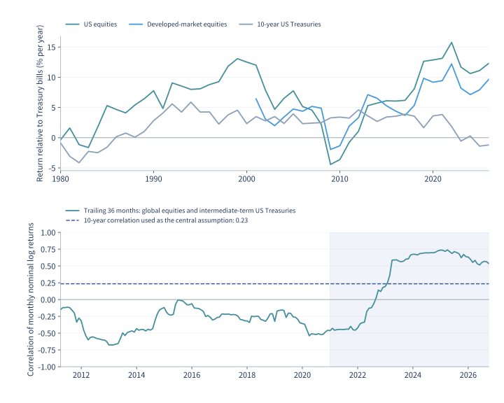
J.P. Morgan projects a 7.5% annual compound return on global equities in its 2027 outlook. Vanguard's September 2026 medians are 5.8% for US equities and 6.0% outside the US[5, 6]. With the US at about 62% of the global market in early 2026[87], weighting the two regional log returns gives Vanguard a global equivalent of about 5.9%, before any diversification benefit. Averaging the two firms' estimates in log terms gives a compound rate of 6.7%. Earnings, dividends, and potential productivity gains from AI investment support the outlooks, while starting valuations and concentration temper them. Both estimates fall below the recent ten-year historical return.
For intermediate-term US Treasuries, J.P. Morgan's 4.6% projection and Vanguard's 4.8% median give about 4.7% a year. Earlier low yields limited interest income, then rising yields pushed down the prices of outstanding fixed-rate bonds[88]. The higher yields available at the forecast date offer more income than bonds paid early in the historical sample.
I estimate Treasury volatility from IEF, which holds US Treasuries with seven to ten years to maturity. Its longer duration makes it more sensitive to interest-rate changes than the broader intermediate-term category in the outlooks.
I annualize the September 2026 one-month bill return of 0.31% from French's data to set the starting short rate. For the long run I use Vanguard's median forecast of 3.7% a year. I estimate how persistent short rates are by fitting a first-order autoregressive model to monthly total returns on the short-term Treasury fund SHV. Its coefficient of 0.89 means that most of a deviation from the long-run rate carries into the next month. For inflation I use monthly changes in the seasonally adjusted US Consumer Price Index for All Urban Consumers[89]. Fitting the same model gives a persistence coefficient of 0.52. The purchasing-power comparison in §1 uses the unadjusted index.
| Asset | Annual compound return | Historical volatility | Return estimate |
|---|---|---|---|
| Bitcoin | Varies by date and market share | 69.2% | Simulated Bitcoin price paths |
| Global equities | 6.7% | 14.7% | J.P. Morgan, Vanguard |
| Intermediate-term US Treasuries | 4.7% | 6.6% | J.P. Morgan, Vanguard |
Bitcoin's historical volatility of 69.2% uses the unadjusted monthly log returns for the common sample. The price model starts with 68.5% volatility in the transformed market share, based on 120 monthly changes through October 2026 after removing the fitted trend. I use the resulting Bitcoin price paths in the portfolio simulation. The historical cross-asset calculations end in September, the last month with a published CPI at the cutoff.
A compound rate \(c\) implies a mean annual log return \(g=\log(1+c)\). With annual volatility \(\sigma\), the diffusion model gives an expected one-year value per dollar of \(\exp(g+\sigma^2/2)\)[90]. For the portfolio results I simulate asset prices, short rates, and inflation together, preserving the persistence of rates and inflation.
From November 1, 2026 to January 1, 2028, investing at the short-term rate gives an annualized nominal expected return of 3.8% and nominal log-return volatility of 1.4%. For the other assets I use the same period and compute real wealth by dividing each path's nominal wealth by its own price-level multiple.
| Asset | Nominal expected return, annualized | Real expected return, annualized | Volatility of real log return, annualized |
|---|---|---|---|
| Bitcoin | 39.8% | 37.5% | 68.2% |
| Global equities | 7.8% | 6.1% | 14.8% |
| Intermediate-term US Treasuries | 4.9% | 3.3% | 7.2% |
I extrapolate equity and Treasury growth beyond the institutions' forecast horizons. Their published ranges describe potential returns and do not estimate my uncertainty about their means. In §5.3 I change the borrowing rate or the correlations while holding the nominal Bitcoin paths and loss probabilities fixed. I run each scenario separately, without assigning it a probability.
The return assumptions by source, month-end fund values, historical statistics, and simulated asset returns give the inputs and results.
- [82] French, Kenneth R., "Data Library: Fama/French Factors and Developed Market Factors," 2026.
- [86] Damodaran, Aswath, "Historical Returns on Stocks, Bonds and Bills," 2026.
- [5] J.P. Morgan Asset Management, "2027 Long-Term Capital Market Assumptions: Press Release," 2026.
- [6] Vanguard, "Vanguard Capital Markets Model Forecasts, September 30, 2026," 2026.
- [87] Dimson, Elroy, Marsh, Paul, Staunton, Mike, "Global Investment Returns Yearbook 2026: Public Summary," 2026.
- [88] SEC, "Investor Bulletin: Fixed Income Investments — When Interest Rates Go Up, Prices of Fixed-Rate Bonds Fall," 2013.
- [89] U.S. Bureau of Labor Statistics, "Consumer Price Index for All Urban Consumers: All Items, Seasonally Adjusted," 2026.
- [90] J.P. Morgan Asset Management, "Long-Term Capital Market Assumptions: Methodology Handbook," 2025.
| Asset | Expected return, annualized | Volatility of log return, annualized |
|---|---|---|
| Bitcoin | 39.8% | 68.2% |
| Global equities | 7.8% | 14.7% |
| Intermediate-term US Treasuries | 4.9% | 6.6% |
Stock–bond correlations across periods
When demand weakens, easier monetary policy can lift bond prices as equities fall. When inflation or supply constraints dominate, rising rates can push both asset prices down. The Bank for International Settlements, the IMF, and the Federal Reserve discuss those shifts[91, 92, 93]. Part of the Federal Reserve analysis relates equity returns to changes in bond yields. A rise in yields implies a fall in bond prices, reversing the direction relevant to bondholders.
| Sample | Correlation coefficient |
|---|---|
| April 2008–December 2020 | −0.28 |
| January 2021–September 2026 | 0.60 |
| October 2016–September 2026 (10 years) | 0.23 |
| October 2021–September 2026 (5 years) | 0.63 |
J.P. Morgan points to spending, tariffs, energy and supply constraints, and investment demand as sources of continuing inflation uncertainty[5]. I use +0.23 as a middle case that spans different inflation and policy environments. In the other cases the equity–Treasury correlation is +0.63 (the last five years) or +0.02 (August 2010 through September 2026, the longest common sample including Bitcoin). A lower correlation gives bonds more scope to offset stock losses.
| Asset | Bitcoin | Global equities | Intermediate-term US Treasuries |
|---|---|---|---|
| Bitcoin | 1.00 | 0.34 | 0.05 |
| Global equities | 0.34 | 1.00 | 0.23 |
| Intermediate-term US Treasuries | 0.05 | 0.23 | 1.00 |
The Bitcoin–equity correlation was +0.34 over ten years and +0.46 over five. Each sensitivity run replaces the entire three-asset correlation matrix with the matrix from the chosen period. Nominal growth assumptions and the size of shocks to prices, short rates, and inflation stay fixed.
The simulation draws shocks to Bitcoin, equities, Treasuries, short rates, and inflation jointly. The last two shocks enter their respective autoregressive models. The correlations among these shocks differ from correlations among one-year simple returns, which I estimate on separate simulated paths. Historical volatility and correlations include past crashes at their observed frequency. Gaussian shocks approximate ordinary market moves and can miss the frequency and size of extremes.
The correlations by period and shock correlations and persistence estimates specify the historical comparisons and the simulation inputs.
- [91] Bank for International Settlements, "The Correlation of Equity and Bond Returns," 2023.
- [92] Adrian, Tobias, Kramer, Johannes, Malik, Sheheryar, "Stock-Bond Diversification Offers Less Protection From Market Selloffs," 2026.
- [93] Li, Canlin, Yoldas, Emre, "Government Bonds’ Safe-Haven Property and Inflationary Pressures," 2026.
- [5] J.P. Morgan Asset Management, "2027 Long-Term Capital Market Assumptions: Press Release," 2026.
5.2. Portfolio choice when bitcoin can go to zero
Expected log wealth with rebalancing and a single total loss
Let \(w_i\) be the amount in asset \(i\) divided by current investable net worth. Each position is nonnegative and the sum can exceed 1. The funding position \(1-\sum_iw_i\) is cash when positive and debt when negative. I assume investors can continuously rebalance to maintain those targets. If bitcoin becomes worthless, its position disappears. The investor maintains the equity and Treasury targets as fractions of the remaining wealth and adjusts the funding position.
With continuous price fluctuations, a constant short rate \(r\), constant instantaneous expected returns \(\mu\), and a constant return covariance matrix per unit time \(\Sigma\), the unconstrained log-growth optimum is \(w_K=\Sigma^{-1}(\mu-r\mathbf1)\), with \(\mathbf1\) a vector of ones. When the entries sum to a positive value, scaling them to sum to 1 gives the tangency portfolio[7, 94]. In my calculation the positions must be nonnegative and Bitcoin's expected return changes, so I integrate conditional expected returns and covariances over the investment horizon.
Suppose Bitcoin survives to the investment date. Let \(T\) be the horizon, \(t\) time since investment, \(\mu_t\) the drift before permanent loss, and \(\Sigma_t\) the instantaneous return covariance matrix. The diagonal matrix \(D_t\) has ones on its diagonal except that the Bitcoin entry becomes zero after loss. The integrated expected excess returns are \(b=E\int_0^T D_t(\mu_t-r_t\mathbf1)\,dt\) and the integrated covariances are \(C=E\int_0^T D_t\Sigma_tD_t\,dt\). With initial wealth of 1 and a loss probability \(q\) over the horizon, the expected logarithm of final wealth is
\[
\boxed{\begin{aligned}
J(w)&=E\int_0^T r_t\,dt+w^\top b\\
&\quad-\frac12w^\top Cw+q\log(1-w_B).
\end{aligned}}
\]
The last term is the effect of the one-time loss. As the Bitcoin fraction \(w_B\) approaches 1, the surviving fraction of wealth \(1-w_B\) approaches zero and its logarithm tends to negative infinity. The optimum therefore keeps Bitcoin below 100% of net worth even when the other positions take total exposure above 100%.Equivalently, let \(e_B\) be the unit vector for Bitcoin and put the first-order loss in the drift integral, \(b_{\rm all}=b-qe_B\). The objective is then
\[
J(w)=E\int_0^T r_t\,dt+w^\top b_{\rm all}-\frac12w^\top Cw
+q\{\log(1-w_B)+w_B\}.
\]
Here the last term corrects for the nonlinear effect of loss on log wealth. The implementation uses the first form, adding the single loss to a drift calculated from ordinary price changes. Adding the full \(q\log(1-w_B)\) term to a drift that already includes the loss would count part of it twice.I use the central loss curve from §4 and assume loss timing is independent of ordinary price fluctuations. Survival weights Bitcoin's excess return and its covariances because the holding ends at loss. For a future decision the investor observes the date and Bitcoin's market value relative to world wealth. I estimate conditional returns and covariances for that state.
I optimized on 65,536 paths and checked the weights on another 65,536 with a different random seed. The largest change in normalized weights was about 1.3 percentage points. Changing the monthly integration rule moved weights by at most 0.006 percentage points, and the solver matched a case with a known analytical solution.
Real final wealth is \(V_T/I_T\), where \(V_T\) is nominal wealth and \(I_T\) is the price-level multiple. The identity \(\log(V_T/I_T)=\log V_T-\log I_T\) explains why a common set of inflation paths gives the same optimal weights for real and nominal log wealth. The nominal short rate varies over time and applies to both cash and borrowing in the central case.
The central calculation assumes frictionless trading and borrowing, with no margin calls, taxes, or withdrawals for living expenses. Ordinary prices fluctuate continuously. Bitcoin's separate permanent loss is the only price jump, and the model assigns no total-loss event to global equities or Treasuries. Section 5.3 tests borrowing at a spread above the short rate.
The strategy and constraints, integrated returns and covariances, and independent numerical checks document the optimization.
- [7] Merton, Robert C., "Lifetime Portfolio Selection under Uncertainty: The Continuous-Time Case," The Review of Economics and Statistics 51(3), 247―257, 1969.
- [94] Markowitz, Harry, "Portfolio Selection," The Journal of Finance 7(1), 77―91, 1952.
5.3. The starting allocation and how it changes
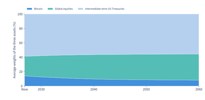
| Asset | Growth-optimal exposure | Same mix, scaled to 100% |
|---|---|---|
| Bitcoin | 47.5% | 14.0% |
| Global equities | 92.4% | 27.3% |
| Intermediate-term US Treasuries | 199.1% | 58.7% |
| Cash or borrowing | −239.0% | 0.0% |
Fractional Kelly sizing and real wealth
Taking a fraction \(f\) of each growth-optimal position \(w_K\) is called fractional Kelly sizing[95]. Cash or borrowing then equals \(1-f\sum_iw_{K,i}\) as a fraction of net worth. If \(L\) is the sum of the growth-optimal positions, scaling them to \(w_K/L\) eliminates borrowing. Here \(f=1/L\) is about 0.29.
| Fraction of full Kelly | Cash (+) or debt (−) as % of net worth | Median final wealth | 10th percentile |
|---|---|---|---|
| 1 (growth-optimal) | −239.0% | 2.80 | 0.51 |
| 1/2 | −69.5% | 2.24 | 0.95 |
| About 0.29 (no borrowing) | 0.0% | 1.80 | 1.08 |
| 1/4 | 15.2% | 1.70 | 1.10 |
I estimate real final wealth on a fresh set of paths with the chosen target fractions maintained for 10.17 years. Full Kelly gives the highest median of the four examples, but at its 10th percentile only about half the starting purchasing power remains.
Maximizing expected log wealth corresponds to relative risk aversion of 1. In the standard model of continuous fluctuations alone, scaling by \(f\) gives the optimum for risk aversion \(1/f\). With permanent loss, fractional Kelly still compares investment scales, but a separate optimization would be needed for each investor's risk aversion. Living expenses and the size of a loss an investor can tolerate also matter.
- [95] Busseti, Enzo, Ryu, Ernest K., Boyd, Stephen, "Risk-Constrained Kelly Gambling," The Journal of Investing 25(3), 118―134, 2016.
Sensitivity to funding costs and return correlations
| Case | Bitcoin | Global equities | Intermediate-term US Treasuries |
|---|---|---|---|
| Central | 14.0% | 27.3% | 58.7% |
| Borrowing rate +0.5 percentage points | 21.9% | 37.0% | 41.1% |
| Borrowing rate +1 percentage point | 41.2% | 58.8% | 0.0% |
| Five-year correlations (Oct. 2021–Sept. 2026) | 20.2% | 18.0% | 61.9% |
| Full-sample correlations (Aug. 2010–Sept. 2026) | 11.2% | 29.5% | 59.3% |
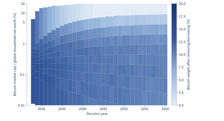
For each row I first maximize log growth with borrowing allowed, then divide each risky position by total risky holdings. A higher funding cost reduces the gain from buying Treasuries with borrowed money. That is why changing the cost of debt can remove them even from the scaled portfolio that carries no debt.
The correlation cases replace the full three-asset matrix with five-year or full-sample estimates. The comparisons preserve the nominal Bitcoin paths and the cumulative loss curve. The results by case also show what happens when the permanent-loss risk is removed.
6. Conclusion
References
- [1] Coin Metrics, "Free Coin Metrics Data Archives," 2026.
- [2] McKinsey Global Institute, "The Global Balance Sheet 2026: Imbalance and Divergence," 2026.
- [3] International Monetary Fund, "World Economic Outlook Database, October 2026," 2026.
- [4] World Gold Council, "Gold Market Primer: Market Size and Structure (Chinese Edition, 18 August 2026)," 2026.
- [5] J.P. Morgan Asset Management, "2027 Long-Term Capital Market Assumptions: Press Release," 2026.
- [6] Vanguard, "Vanguard Capital Markets Model Forecasts, September 30, 2026," 2026.
- [7] Merton, Robert C., "Lifetime Portfolio Selection under Uncertainty: The Continuous-Time Case," The Review of Economics and Statistics 51(3), 247―257, 1969.